July, 17, 2021

Explicit Representation of the Orientation: Exponential Coordinates

In the previous lesson, we became familiar with rotation matrices, and we saw that the nine-dimensional space of rotation matrices subject to six constraints (three unit norm constraints and three orthogonality constraints) could be used to implicitly represent the three-dimensional space of orientations.

There are also methods to express the orientation with a minimum number of parameters (three in three-dimensional space). Exponential coordinates that define an axis of rotation and the angle rotated about that axis, the three-parameter Euler angles, the three-parameter roll-pitch-yaw angles, the Cayley-Rodrigues parameters, and the unit quaternions (use four variables subject to one constraint) are some of the methods to express the orientations with a fewer number of parameters.

In this lesson, we will focus on one of the ways to explicitly represent the space of orientations, namely the exponential coordinates representation. To learn more about implicit and explicit representations of configuration, please refer to this lesson.

This lesson is part of the series of lessons on foundations necessary to express robot motions. For the full comprehension of the Fundamentals of Robot Motions and the necessary tools to represent the configurations, velocities, and forces causing the motion, please read the following lessons (note that more lessons will be added in the future):

https://www.mecharithm.com/category/fundamentals-of-robotics/fundamentals-of-robot-motions/

Also, reading some lessons from the base lessons of the Fundamentals of Robotics course are deemed invaluable.

Exponential Coordinate Representation of Orientation

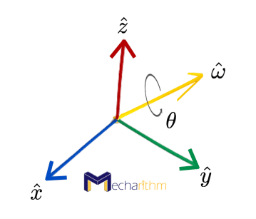
Exponential coordinates of orientation are a three-parameter representation of orientation in which a rotation matrix R can be parameterized in terms of a rotation axis ῶ (a unit vector) and an angle of rotation θ about that axis. If we combine these two parameters, we get the exponential coordinate representation of orientation as:

\[\hat{\omega}\theta \in R^3\]

If we write ῶ and θ individually, we get the axis-angle representation of rotation.

Interpretations for the Exponential Coordinate Representation for a Rotation Matrix

There are three interpretations for the exponential coordinate representation ῶθ for a rotation matrix R:

The axis ῶ and rotation angle θ such that if a frame was initially coincident with the space frame {s} were rotated by θ about ῶ, then its final orientation with respect to {s} can be represented by R.

rotation-about-arbitrary-axis — The Exponential Coordinate Representation of Orientation

See a demo of this interpretation in the video below:

Exponential Coordinate Representation for a Rotation Matrix

If we consider ῶθ as an angular velocity (suppose θ = β̇ ) expressed in {s} frame such that if a frame was initially coincident with {s} and followed ῶθ for one unit of time (in other words it is integrated over this time interval), then its final orientation is expressed by R.

\[\int_{0}^{1} {\hat{\omega} \theta dt} = \hat{\omega} \theta\]

If we consider ῶ to be the angular velocity expressed in {s} (suppose ῶ = φ̇γ̂ ) such that if a frame was initially coincident with {s} followed ῶ for θ units of time (in other words ῶ is integrated over this time interval), then its final orientation can be expressed by R.

\[\int_{0}^{\theta} {\hat{\omega} d\theta} = \hat{\omega} \theta\]

The exponential coordinate representation of orientation got its name because of the link to the linear differential equations.

Some Notes from Linear Differential Equation Theory

From mathematics, we recall that the scalar linear differential equation has the form

\[\dot{x} (t) = ax(t)\]

Where

\[x(t) \in \mathbb{R} ,a \in \mathbb{R} \, \, \text{constant},x(0) = x_0 \, \, \text{initial condition}\]

Then the solution of this scalar linear differential equation is straightforward and can be found

\[x(t) = e^{at} x_0\]

Where the series expansion of the exponential function can be defined as

\[e^{at} = 1 + at + \frac{(at)^2}{2!} + \frac{(at)^3}{3!} + …\]

The scalar case can be generalized to the vector linear differential equations case in the form of

\[\dot{x}(t) = Ax(t)\]

Where

\[x(t)\in {\mathbb{R}}^n, A \in {\mathbb{R}}^{n \times n} \, \, \text{constant}, x(0) = x_0 \, \, \text{initial condition}\]

Then similar to the scalar case, the solution can be expressed in the form

\[x(t) = e^{At} x_0\]

Where the series expansion of the matrix exponential can be expressed as

\[e^{At} = I + At + \frac{(At)^2}{2!} + \frac{(At)^3}{3!} + …\]

Now the question is, what are the conditions that this series converge? The answer can be found in most textbooks on ordinary differential equations, and we bring that up here without proof. If A is constant and finite, then the series is always guaranteed to converge to a finite limit.

With this reminder about the linear differential equations, let’s get back to the exponential coordinate representation of orientation.

Exponential coordinate representation of orientation can be viewed or used in two ways:

A unit axis of rotation ῶ (ῶ ∈ ℝ³, ||ῶ|| = 1) with a rotation angle θ ∈ ℝ about the axis. This representation is called the axis-angle representation and it is useful when representing a robot joint where we can separate the joint axis from the motion θ about the axis.

scara-robot-taskspace-workspace — The SCARA Robot. The three revolute joints rotate about their rotation axes by the corresponding rotation angles. The robot photo is from Wikipedia.

The three-vector ῶθ ∈ ℝ³.

The Analogy between the Exponential Coordinates of Orientation and the Linear Differential Equations

Now let’s see the analogy between the exponential coordinates of orientation and the linear differential equations.

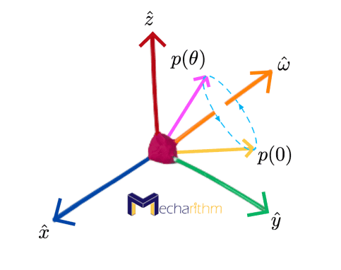
Suppose that a 3-vector p starts from the initial position p(0) and rotates about the rotation axis ῶ by angle θ and reaches the position p(θ). Note the circular path that the vector is traveling. Also, assume that all quantities are expressed in the fixed-frame coordinates:

exponential-coordinates-rotation-circular-path-vectors-about-arbitrary-axis — A vector is rotated about an arbitrary axis to a new location. The vector travels a circular path during travel.

This motion can also be visualized as the video below:

Rotating the vector from the initial location p(0) at time t=0 to the new location p(θ) at time t = θ results in the rate (numerical value) θ̇ to be 1 rad/s.

From the physics of the circular motion, we know that the tip of the vector p(t) traces a circular path during rotation, and we also know that the velocity of p(t) is tangent to the path and can be calculated by the cross product of the angular velocity and the radius vector of the circular path:

exponential-coordinates-circular-path-velocity-tangent — The tip of the vector p(t) traces a circular path during rotation, and the velocity of p(t) is tangent to this circular path and can be calculated by the cross product of the angular velocity and the radius vector of the circular path.

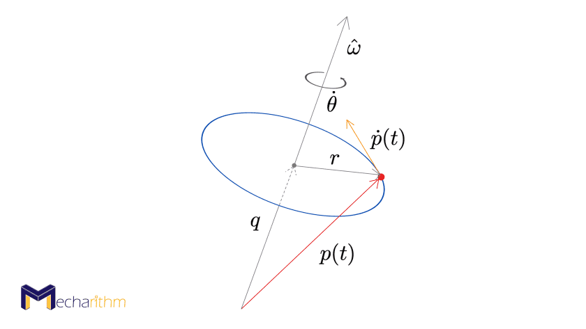
Remember that the velocity has a direction, whereas the speed is a numerical quantity. So the speed can simply be the product of the radius and the rate of the angular velocity.

The velocity of the tip of the vector is calculated as:

\[\dot{p} = \omega \times r\]

The angular velocity ω can simply be calculated as the rate of the angular velocity (in this case, it is one) in the axis of rotation direction:

\[\omega = \hat{\omega} \dot{\theta} = \hat{\omega}\]

And from the geometry, we can write:

\[q+r = p \rightarrow r = p-q\]

Therefore, the velocity of the circular path can be found as:

\[\dot{p} = \hat{\omega} \times (p-q) = \hat{\omega} \times p – \underbrace{\hat{\omega} \times q}_{0}= \hat{\omega} \times p\]

The cross product of ῶ and q is zero since the angle between them is zero.

Physical Demonstration of the Tangent Velocity in Circular Motion

If you like to have a physical understanding of this velocity, consider a salad spinner. When you spin the wet veggies with a known rate, each water droplet goes through a circular path with velocity tangent to the path that causes them to leave the veggies basket:

Tangent velocity to the circular path can be physically visualized by leaving water droplets from the salad basket while going through a circular motion.

Definition of Cross Product between Two Vectors

As a quick reminder that if a,b ∈ ℝ³ are two vectors defined by their coordinates as a = (a₁,a₂,a₃), b = (b₁,b₂,b₃), and the angle between the two vectors is θ

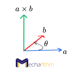
exponential-coordinate-orientation-cross-product — The cross product of the two vectors is perpendicular to the plane containing a and b, and the direction follows the right-hand rule.

then the cross product of the two vectors can be defined in two ways

the cross product can be calculated by the formal determinant as

\[a \times b = \begin{vmatrix}\hat{x} & \hat{y} & \hat{z}\\a_1 & a_2 & a_3 \\b_1 & b_2 & b_3\end{vmatrix} = (a_2 b_3 – a_3 b_2)\hat{x} + (a_3 b_1 – a_1 b_3)\hat{y} + (a_1 b_2 – a_2 b_1) \hat{z}\]

it can also be calculated by the product of the magnitudes of the two vectors and the sine of the angle between them in the direction of the unit vector perpendicular to the plane containing a and b in a right-handed frame

\[a \times b = ||a|| ||b|| sin \theta \hat{n}\]

Remember that the cross product of b and a is in the opposite direction of the cross product between a and b

\[b \times a = – a \times b\]

Now let’s go back to the analogy between the Exponential Coordinates of Orientation and the Linear Differential Equations. Using the skew-symmetric representation, we can change the equation for the tangent velocity described above to a linear differential equation of the form

\[\dot{p} = \hat{\omega}\times p = [\hat{\omega}]p, \quad p(0) \, \, \text{initial condition}\]

Where the [ῶ] is the skew-symmetric matrix representation of the vector ῶ.

By definition, if we have a vector defined as

\[a = \begin{bmatrix}a_1 & a_2 & a_3\end{bmatrix} ^ T \in {\mathbb{R}}^3\]

Then, the 3×3 skew-symmetric matrix representation of a can be defined as

\[[a] = \begin{bmatrix}0 & -a_3 & a_2\\a_3 & 0 & -a_1\\-a_2 & a_1 & 0\end{bmatrix}\]

Note that since [a] is a skew-symmetric matrix, then:

\[[a] = -[a]^T\]

The solution to our linear differential equation, as we saw before, can be expressed as

\[p(t) = e^{[\hat{\omega}]t}p(0)\]

And since t and θ are interchangeable here, we can write

\[p(\theta) = e^{[\hat{\omega}]\theta}p(0)\]

From this equation, we can see that the matrix exponential is the transformation that rotates the initial vector about an axis to the final position, and thus it is the rotation matrix R (see different applications of a rotation matrix in this lesson). Now let’s see if we can find a closed-form solution for this matrix exponential. From the series expansion that we saw before, we can write

\[\begin{split}e^{[\hat{\omega}]\theta} & = I + [\hat{\omega}]\theta + [\hat{\omega}]^2 \frac{\theta^2}{2!} + [\hat{\omega}]^3 \frac{\theta^3}{3!} + … \\& = I + [\hat{\omega}]\theta + [\hat{\omega}]^2 \frac{\theta^2}{2!} – [\hat{\omega}] \frac{\theta^3}{3!} – [\hat{\omega}]^2 \frac{\theta^4}{4!} + [\hat{\omega}] \frac{\theta^5}{5!} + …\\& = I + (\theta – \frac{\theta^3}{3!} + \frac{\theta^5}{5!} – …)[\hat{\omega}] + (\theta^2 – \frac{\theta^4}{4!} + \frac{\theta^6}{6!} – …)[\hat{\omega}]^2\\& = I + sin \theta [\hat{\omega}] + (1-cos \theta)[\hat{\omega}]^2\end{split}\]

This equation was derived with the help of the following equations

\[[\hat{\omega}]^4 = -[\hat{\omega}]^2\\ [\hat{\omega}]^5 = -[\hat{\omega}]^3 = [\hat{\omega}] \\. \quad \quad \quad\\.\quad \quad \quad\\. \quad \quad \quad\]

and the series expansions for sine and cosine

\[\begin{cases} sin\theta = \theta – \frac{\theta^3}{3!} + \frac{\theta^5}{5!} – …\\ cos\theta = 1 – \frac{\theta^2}{2!} + \frac{\theta^4}{4!} – …\end{cases}\]

The above formula for the matrix exponential is called Rodrigues’s formula for rotations, and it uses the matrix exponential to construct a rotation matrix from a rotation axis ῶ and an angle θ. Formally we can define this as

Given a vector ῶθ ∈ ℝ³ in which θ is any scalar and ῶ ∈ ℝ³ is a unit vector, then the matrix exponential of

\[[\hat{\omega}] \theta = [\hat{\omega} \theta ] \in so(3)\]

\[Rot(\hat{\omega},\theta) = e^{[\hat{\omega}]\theta} = I + sin \theta [\hat{\omega}] + (1-cos\theta)[\hat{\omega}]^2 \in SO(3)\]

This is the same formula we saw in the previous lesson when we talked about the general formula for rotation operators. It takes a 3×3 so(3) representation of exponential coordinates and calculates R in SO(3) that is achieved by rotating about ῶ by θ from an initial orientation R = I.

Therefore we can say that the matrix exponential above can act as an operator and rotate a frame or a vector. So

\[e^{[\hat{\omega}]\theta} p\]

can rotate the vector p ∈ ℝ³ about the fixed frame axis ῶ by an angle θ. Also, if R is a rotation matrix with three column vectors, then

\[R’ = e^{[\hat{\omega}]\theta} R = Rot(\hat{\omega},\theta)R\]

is the orientation archived by rotating R by θ about the axis ῶ in the fixed frame and

\[R” = Re^{[\hat{\omega}]\theta} = RRot(\hat{\omega},\theta)\]

is the orientation achieved by rotating R by θ about the axis ῶ in the body frame.

The matrix exponential rakes the skew-symmetric representation of exponential coordinates ῶθ and calculates the corresponding rotation matrix:

Exponentiation: [ῶ]θ ∈ so(3) → R ∈ SO(3)

The set of all 3×3 real skew-symmetric matrices is called so(3), which is called the Lie algebra of the Lie group SO(3). In general, the space of n×n skew-symmetric matrices is called so(n) and can be defined as

so(n) = {S ∈ ℝ^n×n: S^T = -S}

Matrix Logarithm of Rotations

For any rotation matrix R ∈ SO(3), we can always find a unit vector ῶ and scalar θ such that R = e^[ῶ]θ. This brings up a new discussion about the matrix logarithm of rotations. The matrix logarithm is the inverse of the matrix exponentiation discussed above. In fact, the matrix exponentiation “integrates” the matrix representation of an angular velocity [ῶ]θ ∈ so(3) for one second to give an orientation R ∈ SO(3). On the other hand, matrix logarithm “differentiates” an R ∈ SO(3) to find the matrix representation of a constant angular velocity [ῶ]θ ∈ so(3) which, if integrated for one second, could rotate a frame from I to R.

In summary

\[\begin{cases} exp: [\hat{\omega}]\theta \in so(3) \rightarrow R \in SO(3)\\ log: R\in SO(3) \rightarrow [\hat{\omega}]\theta \in so(3) \end{cases}\]

So, now the problem is if we have the rotation matrix R ∈ SO(3) as

\[R = \begin{pmatrix}r_{11} & r_{12} & r_{13}\\r_{21} & r_{22} & r_{23} \\r_{31} & r_{32} & r_{33}\end{pmatrix}\]

What are the corresponding ῶ = (ῶ₁,ῶ₂,ῶ₃), and θ? In order to find these, we need to equate the matrix exponential formula to the rotation matrix defined above

\[e^{[\hat{\omega}]\theta} = I + sin\theta [\hat{\omega}] + (1-cos\theta){[\hat{\omega}]}^2 = \begin{pmatrix}c_{\theta} + {\hat{\omega}_1}^2(1-c_{\theta}) & \hat{\omega}_1 \hat{\omega}_2 (1-c_{\theta}) – \hat{\omega}_3 s_{\theta} & \hat{\omega}_1 \hat{\omega}_3 (1-c_{\theta}) + \hat{\omega}_2 s_{\theta}\\\hat{\omega}_1 \hat{\omega}_2 (1-c_{\theta}) + \hat{\omega}_3 s_{\theta} & c_{\theta} + {\hat{\omega}_2}^2 (1-c_{\theta}) & \hat{\omega}_2 \hat{\omega}_3 (1-c_{\theta}) – \hat{\omega}_1 s_{\theta}\\\hat{\omega}_1 \hat{\omega}_3 (1-c_{\theta}) – \hat{\omega}_2 s_{\theta} & \hat{\omega}_2 \hat{\omega}_3 (1-c_{\theta}) + \hat{\omega}_1 s_{\theta} & c_{\theta} + {\hat{\omega}_3}^2 (1-c_{\theta})\end{pmatrix} \\= \begin{pmatrix}r_{11} & r_{12} & r_{13}\\r_{21} & r_{22} & r_{23} \\r_{31} & r_{32} & r_{33}\end{pmatrix}\]

Where s_θ = sinθ, c_θ = cosθ.

By subtracting the transpose of each matrix from both sides, we can get

\[\begin{cases}r_{32} – r_{23} = 2 \hat{\omega}_1 sin \theta\\r_{13} – r_{31} = 2 \hat{\omega}_2 sin \theta\\r_{21} – r_{12} = 2 \hat{\omega}_3 sin \theta\end{cases}\]

As long as θ is not an integer multiple of π that is sin θ ≠ 0, we can write the above equations as

\[\begin{cases}\hat{\omega}_1 = \frac{1}{2sin \theta} (r_{32} – r_{23})\\\hat{\omega}_2 = \frac{1}{2sin \theta} (r_{13} – r_{31})\\\hat{\omega}_3 = \frac{1}{2sin \theta} (r_{21} – r_{12})\end{cases}\]

Expressing these equations in skew-symmetric matrix form, we can get

\[[\hat{\omega}] = \begin{pmatrix}0 & -\hat{\omega}_3 & \hat{\omega}_2\\\hat{\omega}_3 & 0 & -\hat{\omega}_1 \\-\hat{\omega}_2 & \hat{\omega}_1 & 0\end{pmatrix} = \frac{1}{2sin \theta} \begin{pmatrix}r_{11} & r_{12} & r_{13}\\r_{21} & r_{22} & r_{23} \\r_{31} & r_{32} & r_{33} \end{pmatrix} – \begin{pmatrix}r_{11} & r_{21} & r_{31}\\r_{12} & r_{22} & r_{32}\\ r_{13} & r_{23} & r_{33} \end{pmatrix} = \frac{1}{2sin \theta} (R – R^T)\]

ῶ gives the axis of rotation for the given R.

[ῶ] is not well-defined if θ is an integer multiple of π, and those angels are called the singularities of the representation. As we saw in the Configuration and Configuration Space lesson, singularities are unavoidable for any 3-parameter representation of orientation. Euler angles and roll-pitch-yaw angles have the same singularities.

Now assume that sinθ ≠ 0, and we want to find an expression for θ. We equate the known rotation matrix R to the matrix exponential from Rodrigues’s formula:

\[R = e^{[\hat{\omega}]\theta} \rightarrow \begin{pmatrix}r_{11} & r_{12} & r_{13}\\r_{21} & r_{22} & r_{23} \\r_{31} & r_{32} & r_{33} \end{pmatrix} = \begin{pmatrix}c_{\theta} +{\hat{\omega}_1}^2 (1-c_{\theta}) & \hat{\omega}_1 \hat{\omega}_2 (1-c_{\theta}) – \hat{\omega}_3 s_{\theta} & \hat{\omega}_1 \hat{\omega}_3 (1-c_{\theta}) + \hat{\omega}_2 s_{\theta}\\\hat{\omega}_1\hat{\omega}_2 (1-c_{\theta}) + \hat{\omega}_3 s_{\theta} & c_{\theta} + {\hat{\omega}_2}^2 (1-c_{\theta}) & \hat{\omega}_2 \hat{\omega}_3 (1-c_{\theta}) – \hat{\omega}_1 s_{\theta} \\\hat{\omega}_1 \hat{\omega}_3 (1-c_{\theta}) -\hat{\omega}_2 s_{\theta} & \hat{\omega}_2 \hat{\omega}_3 (1-c_{\theta}) + \hat{\omega}_1 s_{\theta} & c_{\theta} + {\hat{\omega}_3}^2 (1-c_{\theta})\end{pmatrix}\]

By taking the trace of both sides (remember that the trace of a matrix is the sum of diagonal terms), we get

\[r_{11} + r_{22} + r_{33} = 3c_{\theta} + (1-c_{\theta}) \underbrace{({\hat{\omega}_1}^2 + {\hat{\omega}_2}^2 +{\hat{\omega}_3}^2 )}_{=1} = 1 + 2c_{\theta}\]

For any θ satisfying this equation such that θ is not an integer multiple of π, and [ῶ] defined above, R can be expressed as the exponential matrix e^[ῶ]θ.

Now let’s discuss the case where θ = kπ and k is some integer.

Case 1: k is an even integer, then no mater what the axis of rotation ῶ is, we have rotated back to R = I so the vector ῶ is undefined.
Case 2: k is an odd integer (θ = ±π, ±3π, …), then tr R = -1, and R = e^[ῶ]θ = I + 2[ῶ]² (from Rodrigues’s formula). Expanding this expression for R we get

\[\begin{pmatrix}2{\hat{\omega}_1}^2 – 1 & 2\hat{\omega}_1\hat{\omega}_2 & 2\hat{\omega}_1\hat{\omega}_3\\2\hat{\omega}_1\hat{\omega}_2 & 2{\hat{\omega}_2}^2 – 1 & 2\hat{\omega}_3\hat{\omega}_2\\2\hat{\omega}_1 \hat{\omega}_3 & 2 \hat{\omega}_2 \hat{\omega}_3 & 2{\hat{\omega}_3}^2 – 1\end{pmatrix} =\begin{pmatrix}r_{11} & r_{12} & r_{13}\\r_{21} & r_{22} & r_{23}\\r_{31} & r_{32} & r_{33}\end{pmatrix}\]

and thus

\[\begin{cases}2 {\hat{\omega}_1}^2 – 1 = r_{11}\\2 {\hat{\omega}_2}^2 – 1 = r_{22}\\2 {\hat{\omega}_3}^2 – 1 = r_{33}\end{cases} , \begin{cases}r_{12} = r_{21} = 2 \hat{\omega}_1 \hat{\omega}_2\\r_{13} = r_{31} = 2 \hat{\omega}_1 \hat{\omega}_3\\r_{23} = r_{32} = 2 \hat{\omega}_2 \hat{\omega}_3\end{cases}\]

We can see that R is symmetric since R^T = R. Thus, in summary, from diagonal terms, we can write:

\[\hat{\omega}_i = \pm \sqrt{\frac{r_{ii}+1}{2}}, \, \, i = 1,2,3\]

and from off-diagonal terms:

\[\begin{cases}2\hat{\omega}_1 \hat{\omega}_2 = r_{12}\\2\hat{\omega}_2 \hat{\omega}_3 = r_{23}\\2\hat{\omega}_1 \hat{\omega}_3 = r_{13}\end{cases}\]

and because of the symmetry of R:

\[\begin{cases}r_{12} = r_{21}\\r_{13} = r_{31}\\r_{23} = r_{32}\end{cases}\]

These equations are used to find a solution for ῶ and once such a solution is found, then R = e^[ῶ]θ where θ = ±π, ±3π, …

Remember that if ῶ is a solution, so is -ῶ (this is only true for this case).

So in summary, if we are given R ∈ SO(3), using the approach above, we can find a θ and a unit rotation axis ῶ ∈ ℝ³, ||ῶ|| = 1 such that e^[ῶ]θ = R. The vector ῶθ ∈ ℝ³ is the exponential coordinate of R and the skew-symmetric matrix [ῶ]θ ∈ so(3) is the matrix logarithm of R.

Since every R ∈ SO(3) satisfies one of the conditions above, for every R, there exist a matrix logarithm [ῶ]θ and therefore a set of exponential coordinates ῶθ.

Example:

If the rotation matrix R is defined by successive rotations about the z-axis of the space frame by 180^o followed by a rotation about the x-axis of the space frame by 90^o as (notice the order in which the rotations are written)

\[R = Rot(\hat{x},90^{o}) Rot(\hat{z},180^{o}) = \begin{pmatrix}-1 & 0 & 0\\0 & 0 & -1\\0 & -1 & 0\end{pmatrix}\]

The rotation operators about the x and z axes used in this calculation can be found in this lesson. If you like to visualize this rotation, you can watch the following demonstration and verify that the orientation of the final frame with respect to the base frame is indeed the rotation matrix above

We want to find a unit vector ῶ and an angle θ such that R = e^[ῶ]θ.

From the expression that we found for R, we can see that tr R = -1, and we can write

\[-1 = 1+2cos \theta \rightarrow cos \theta = -1 \rightarrow \theta = \pi (\text{or} \, 180^{0})\]

So, we are dealing with case 2 that by checking the conditions, we can say that

\[\hat{\omega} = \frac{1}{\sqrt2} \begin{pmatrix}0\\-1 \\1\end{pmatrix}, \text{or} \, \frac{1}{\sqrt2} \begin{pmatrix}0\\1 \\-1\end{pmatrix}\]

Remember that if ῶ is a solution, so is the -ῶ.

So, the orientation of the frame achieved by a rotation from the initial orientation about ῶ calculated above by an angle 180⁰ gives the same orientation as the frame if it was rotated first about the z-axis of the space frame by 180^o followed by a rotation about the x-axis of the space frame by 90^o.

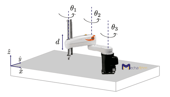
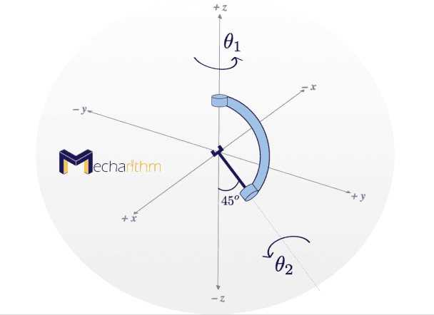
Demonstration: The Orientation of a Two Degrees of Freedom Robot Wrist

Consider a 2-DOF robot wrist mechanism in zero position (all joint angles are set to zero) depicted in the following figure

exponential-coordinate-orientation-two-dof-robot-wrist — A two-dof robot wrist mechanism is depicted in the zero position (all joint angles are set to zero).

If you are not familiar with the degrees of freedom for a robot, you can check the lesson named Everything About the Degrees of Freedom of a Robot first.

From the above figure, we can see that the axis of rotation of the first joint can be written as

\[\hat{\omega}_{j1} = \begin{pmatrix}0\\0 \\1\end{pmatrix}\]

Which is the z-axis, and the axis of rotation of the second joint can be found as

\[\hat{\omega}_{j2} = \begin{pmatrix}0\\cos45^{o} \\-cos45^{o}\end{pmatrix} = \begin{pmatrix}0\\\frac{\sqrt 2}{2}\\-\frac{\sqrt 2}{2}\end{pmatrix}\]

Thus the orientation of the gripper R ∈ SO(3) can simply be calculated by the product of matrix exponentials and expanding the matrix exponentials using Rodrigues’s formula and inserting the values for the axes of rotation as

\[R = e^{[\hat{\omega}_{j1}]\theta_1} e^{[\hat{\omega}_{j2}]\theta_2} = \begin{pmatrix}c_{\theta_1} & -s_{\theta_1} & 0\\s_{\theta_1} & c_{\theta_1} & 0 \\0 & 0 & 1\end{pmatrix} \begin{pmatrix}c_{\theta_2} & \frac{1}{\sqrt 2} s_{\theta_2} & \frac{1}{\sqrt 2} s_{\theta_2}\\-\frac{1}{\sqrt 2} s_{\theta_2} & \frac{1}{2} (c_{\theta_2} + 1) & \frac{1}{2} (c_{\theta_2} – 1) \\-\frac{1}{\sqrt 2} s_{\theta_2} & \frac{1}{2} (c_{\theta_2} – 1) & \frac{1}{2} (c_{\theta_2} + 1)\end{pmatrix}\]

Now the question is, is there any set of angels (θ₁, θ₂) so that in those positions, the following orientation R can be achieved? (in other words, can this mechanism reach this orientation?)

\[R = \begin{pmatrix}\frac{1}{\sqrt 2} & 0 & -\frac{1}{\sqrt 2}\\0 & 1 & 0\\\frac{1}{\sqrt 2} & 0 & \frac{1}{\sqrt 2}\end{pmatrix}\]

If we take the third row of the product of matrix exponentials, then set it equal to the third row of R

\[\begin{pmatrix}-\frac{1}{\sqrt 2} s_{\theta_2} & \frac{1}{2} (c_{\theta_2} – 1) & \frac{1}{2} (c_{\theta_2} + 1) \end{pmatrix} = \begin{pmatrix}\frac{1}{\sqrt 2} & 0 & \frac{1}{\sqrt 2} \end{pmatrix}\]

By inspection, we can see that there is no θ₂ that satisfies this equation, and thus the wrist mechanism above cannot reach that orientation.

That’s going to wrap up today’s lesson. In the next lesson, we will learn about other explicit representations of orientation.

The video version of the current lesson can be watched at the link below:

References:
📘 Textbooks:
Modern Robotics: Mechanics, Planning, and Control by Frank Park and Kevin Lynch
A Mathematical Introduction to Robotic Manipulation by Murray, Lee, and Sastry

✍️ Logo design by Minro Art Group