Holonomic vs. Nonholonomic Constraints for Robots
In this post, you will learn that holonomic or configuration constraints reduce the degrees of freedom (dofs) of a robot, whereas nonholonomic constraints reduce the space of possible velocities.
⚠️ This post also has a video version that complements the reading. Our suggestion is to watch the video and then read the reading for a deeper understanding.
Holonomic (Configuration) Constraints for Robots
Let’s see this with an example. Remember our famous 4-bar linkage with one degree of freedom? If you do not, please refer to this lesson.
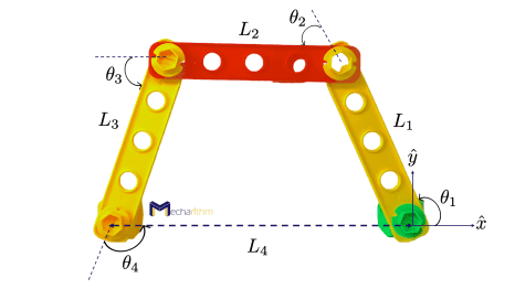
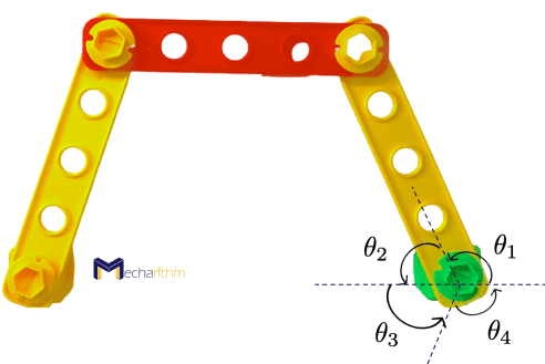
For now, consider a 4-bar linkage that has 4 links (ground is a link, remember?) that has one DOF and the two ends are pinned to the ground:
Since it has one degree of freedom, then the configuration space (C-space) has one dimension. For a complete lesson on configuration space, including topology and representation, click HERE!
It is super difficult to represent the configuration space with only one parameter. A viable option is an implicit representation of the C-space that is embedding the configuration space in a higher dimensional Euclidean space subject to constraints.
The best common approach to represent the C-space of the closed-loop mechanisms is to represent the C-space by the joint angles subject to loop closure constraints. These constraints are called holonomic constraints, and they will reduce the number of degrees of freedom of a mechanism.
For the 4-bar linkage example, the configuration space can be represented by:
Subject to three-loop closure constraints.
In order to find the loop constraints note that:
- The tip of link 4 always coincides with the origin
- The orientation of link 4 is always horizontal
We can also visualize this with a 4-link serial robot that satisfies the above conditions:
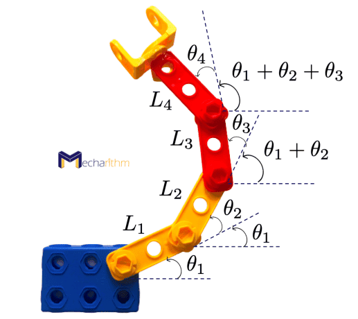
The three loop-closure equations can then be written as:
The final position and orientation after going around the loop are equal to the initial position and orientation:
These loop closure equations are called holonomic constraints and reduce the C-space dimension and thus the degrees of freedom of a mechanism.
Therefore the one-dimensional (1D) C-space can be implicitly represented by embedding in a four-dimensional (4D) space of joint angles subject to three constraints.
If we write the n-D vector of the robot’s configuration as:
Then the loop closure equations for k independent equations (= k holonomic constraints) can be written in vector form as follows:
The k independent constraints are called holonomic, or configuration constraints and they are constraints that reduce the dimension of the C-space.
Then the dimension of the C-space or degrees of freedom is:
Velocity (Pfaffian) Constraints
If the robot is moving and follows the time trajectory q(t), then the question is how do these holonomic constraints restrict the velocity of the robot?
If we write:
Then differentiating both sides with respect to t:
Which can then be written as follows:
Re-writing this equation:
In which q̇i is the joint i velocity.
The equation:
is called the velocity or Pfaffian constraints. There are two conditions here:
- If the velocity constraints are integrable, then they are called holonomic or integrable, or configuration constraints.
- If the velocity constraints cannot be integrated to get the configuration constraints, they are called nonholonomic constraints.
Nonholonomic Constraints
Now let’s see some examples for nonholonomic constraints:
Example 1: Chassis of a Car Driving on a Plane
Suppose a chassis of a car driving on a plane:
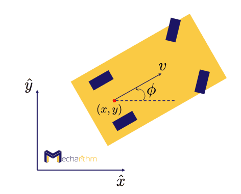
Where ϕ is the chassis angle (steering angle). A sample path of the car depending on this angle can be like this:
(x,y) is the location of the point halfway between the rear wheels. v is the forward velocity of the car.
Then the configuration of the chassis can be determined by:
In order to find the velocities in x and y direction, we can write:
From second equation we can write that:
Substituting this equation into the first equation we can write:
Re-writing this equation in the form of the Pfaffian constraints, we can get the following equation:
This velocity constraint cannot be integrated to give an equivalent configuration constraint, and thus it is a nonholonomic constraint.
Example 2: Steerable Needles
Steerable Needles are a type of medical device that can be steered to reach a target location.
Steerable Needles are also an example of nonholonomic systems where they cannot instantaneously reach sideways motions but can be steered to any configuration in their configuration space.
Example 3: A Coin Rolling on a Plane without Slipping (A Classical Problem)
Consider a coin with a radius r rolling on a plane without slipping:
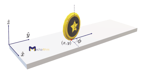
Where
r is the radius of the coin
(x,y) is the contact point of the coin with the plane
ϕ is the rotation around z which is also called steering angle or heading angle
θ is the rotation around x which is also orientation with respect to vertical
The disk has two holonomic constraints that reduce the C-space dimension, and thus it will have four degrees of freedom (6 – 2 = 4). The holonomic constraints are as follows:
- The disk is confined to the x-y plane and cannot move in the z-direction
- Rotating the disk around y will make it lose its upright position
Thus the 4D C-space of the rolling coin can be written as follows:
We remember from the lesson on Configuration Space and Topology that the Cartesian product of two circles is the torus’s 2D surface, which is parameterized by angles ϕ and θ here.
From physics, we know that the coin rolls in the direction indicated by (cosϕ,sinϕ) with the forward speed rθ̇. Thus we can write the velocities in x and y direction as:
If we take the 4D C-space coordinates as:
Then the Pfaffian constraints can be written as follows:
These Pfaffian constraints are not integrable, and thus they are nonholonomic constraints. This means that for the A(q) there is not a differentiable function g: R4 → R2 such that:
Two prove this; we can say that if that had not been the case, there should have existed differentiable g1(q) and g2(q) that could have satisfied the following equalities:
By inspection, we can see that no such g1(q) exists. The same procedure is applicable for g2(q). Thus the Pfaffian constraints are not integrable, and thus these are nonholonomic constraints.
These constraints reduce the dimension of the system’s feasible velocities but do not reduce the dimension of the reachable C-space. The rolling coin can reach any point in its 4D C-space despite the two constraints on its velocity. We will see later in the control section that we will have two velocities to control.
Note that nonholonomic constraints arise in robot systems subject to conservation of momentum or rolling without slipping.
Important Notes on Nonholonomic Constraints
Nonholonomic constraints:
- Reduce the vehicle’s possible velocities (car, steerable needle, etc.), which means that the vehicle cannot slide directly to the side.
- Cannot reduce the space of configurations, which means that for the example of the car, sideway motions can be achieved by parallel parking, or for the case of steerable needles, they can be steered to the desired place. The vehicle can reach any configuration in its 3D space.
A rigid body (for example, a robot) in space can be subject to holonomic and nonholonomic constraints. For the example of the chassis of the car moving on a plane, we can say that:
- It has three holonomic constraints that keep the chassis confined to the plane (we have seen this in the previous lesson HERE).
- It has one nonholonomic constraint that prevents sideways sliding.
Summary of the Holonomic and Nonholonomic Constraints
- Holonomic constraints are constraints on the configuration, and they reduce the space of the configurations and thus the degrees of freedom.
- Nonholonomic constraints are constraints on the velocity, and they do not reduce the space of configurations.
- Pfaffian constraints can be holonomic or nonholonomic based on the integrability of the velocity constraints.
References:
Textbooks:
- Modern Robotics: Mechanics, Planning, and Control by Frank Park and Kevin Lynch
A Mathematical Introduction to Robotic Manipulation by Murray, Lee, and Sastry