Implementing Dynamics and Control of a Quadrotor in MATLAB
In this post, we will implement the dynamics and control of a quadrotor in MATLAB and Simulink. Stabilizing and tracking controllers are simulated and implemented on Quadcopter. A square trajectory is specified for the tracking controller.
The reference of the simulation equations is the paper “Modeling and control of quadcopter” by Teppo Luukkonen.
You can download the paper HERE! It has a table of values that we will use for the simulation.
Objective: Simulation of Dynamics and Control of a Quadrotor in MATLAB and Simulink
The objective is to implement a simulation of the quadcopter dynamics by implementing the equations of motion given in the paper. We will then:
- Implement the stabilizing controller using the gains given in the paper.
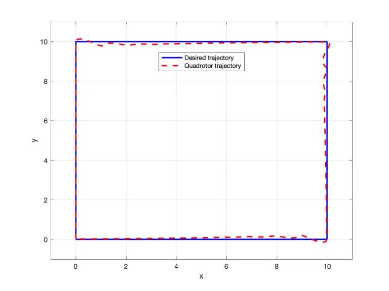
- Implement a controller to follow a square trajectory with the body-fixed x-axis aligned with the direction of travel.
Solution for Simulation of Dynamics and Control of a Quadrotor in MATLAB and Simulink
The following stabilizing controller and tracking controller are implemented in Simulink:
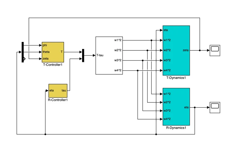
The main program to get the outputs for stabilizing controller and tracking controller for the quadcopter is as follows:
%the main program
clc
clear
close all
% quadcopter Parameters
% parameters of the system
g = 9.81; % gravity constant m/s^2
m = 0.468; % mass of helicopter kg
l = 0.225; % distance between a rotor and the center of quadcopter (m)
k = 2.98e-6; % lift constant
b = 1.14e-7; % drag constant
I_M = 3.357e-5; % rotational moment of inertia kg.m^2
% drag force coefficients
A_x = 0.25; % kg/s
A_y = 0.25;
A_z = 0.25;
% inertia matrix
I_xx = 4.856e-3; %kgm^2
I_yy = 4.856e-3;
I_zz = 8.801e-3;
% parameters of the PD controller
KpT = 3.5;
KdT = 4.5;
KpR = 1;
KdR = 3;
%%%%%%%%%%%%%%%%%%%%%%%%%%%%%%%%%%%%%%%%
% simulation parameters
T_f = 0.01; % simulation interval
% AT = 1e-6; % absolute tolerance
% RT = 1e-6; % relative tolerance
% RF = 4; % Refine factor
%%%%%%%%%%%%%%%%%%%%%%%%%%%%%%%%%%%%%%%
% start simulation
sim('Quadrotor_Stabilization')
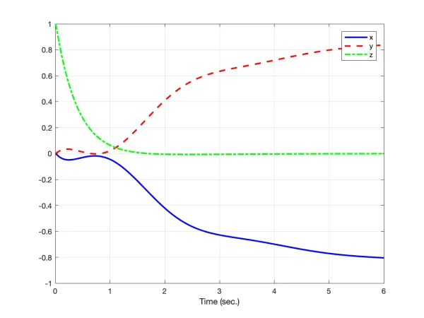
figure
h1 = plot(Time, x, 'b', 'linewidth',2);
hold on
h2 = plot(Time, y, 'r', 'linewidth',2, 'LineStyle', '--');
h3 = plot(Time, z, 'g', 'linewidth',2, 'LineStyle', '-.');
legend([h1 h2 h3], 'x', 'y', 'z')
grid on
xlabel('Time (sec.)');
figure
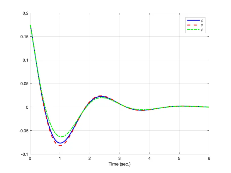
h1 = plot(Time, phi, 'b', 'linewidth',2);
hold on
h2 = plot(Time, theta, 'r', 'linewidth',2, 'LineStyle', '--');
h3 = plot(Time, psi, 'g', 'linewidth',2, 'LineStyle', '-.');
legend([h1 h2 h3], '\phi', '\theta', '\psi')
grid on
xlabel('Time (sec.)');
%%
sim('Quadrotor_Tracking')
% figure
% plot3(xd,yd,1*ones(length(xd)), 'b', 'linewidth', 2);
% hold on
% plot3(x,y,1*ones(length(x)), 'r', 'linewidth',2);
% xlabel('x')
% ylabel('y')
% zlabel('z')
% grid on
figure
h1 = plot(xd, yd, 'b', 'linewidth',2);
hold on
h2 = plot(x, y, 'r', 'linewidth', 2, 'LineStyle', '--');
legend([h1 h2], 'Desired trajectory', 'Quadrotor trajectory', 'Location', 'best')
axis([-1 11 -1 11])
grid on
xlabel('x');
ylabel('y');By running this code we will get the following results for stabilizing controller, and tracking controller of the quadcopter as follows:
- You can download the codes to get the above results HERE!