July, 02, 2021

Implicit Representation of the Orientation: a Rotation Matrix

In the previous lesson, we became familiar with the concept of the configuration for the robots, and we saw that the configuration of a robot could be expressed by the pair (R,p) in which R is the rotation matrix that implicitly represents the orientation of the body frame with respect to the reference frame and p is the position of the origin of the body frame relative to the space frame.

In this lesson, we will focus on the orientation, and we will see that we can implicitly represent the orientation using powerful tools named rotation matrices, and we will understand everything about rotation matrices and their properties and various uses.

This lesson is part of the series of lessons on foundations necessary to express robot motions. For the full comprehension of the Fundamentals of Robot Motions and the necessary tools to represent the configurations, velocities, and forces causing the motion, please read the following lessons (note that more lessons will be added in the future):

https://www.mecharithm.com/category/fundamentals-of-robotics/fundamentals-of-robot-motions/

Also, reading some lessons from the base lessons of the Fundamentals of Robotics course are deemed invaluable.

Introduction to Rotation Matrices

In the lesson about the degrees of freedom of a mechanism, we learned that we need three parameters to explicitly represent a rigid body’s orientation (rotations around the x, y, and z axes). One implicit way to represent the orientation of a rigid body is using 3×3 rotation matrices (note that this is one of the applications of the rotation matrix) to express the orientation of the body frame relative to the base frame. With the 9-dimensional space of the 3×3 rotation matrices subject to 6 constraints, we can implicitly represent the 3-dimensional space of orientations. In other words, of these 9 parameters, only 3 can be chosen independently. The reason that we opt for implicit representation is to take advantage of the algebraic calculations on matrices.

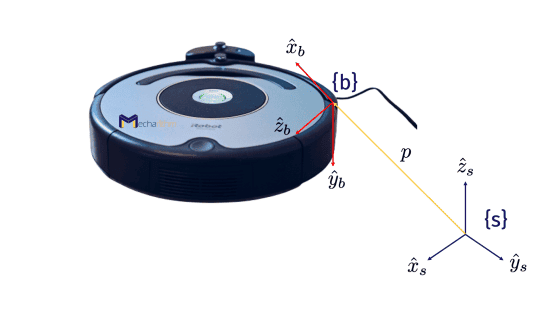
In the previous lesson, we saw the rotation matrix describing the orientation of a toy car on the plane. Now let’s derive a similar representation for the orientation of a robot in space. Suppose a robot in space as shown in the figure below where {b} is the stationary body frame instantaneously attached to the moving body and {s} is the space or reference frame:

representation-robot-motion-space — A Robot in space. {b} is the body frame instantaneously attached to the moving body and {s} is the space or reference frame.

The rotation matrix R can be defined as a representation of the body frame unit axes expressed in the base frame as:

\[R = \begin{bmatrix}\hat{x}_b & \hat{y}_b & \hat{z}_b\end{bmatrix} = \begin{pmatrix}\hat{x}_b.\hat{x}_s & \hat{y}_b.\hat{x}_s & \hat{z}_b.\hat{x}_s\\\hat{x}_b.\hat{y}_s & \hat{y}_b.\hat{y}_s & \hat{z}_b.\hat{y}_s\\\hat{x}_b.\hat{z}_s & \hat{y}_b.\hat{z}_s & \hat{z}_b.\hat{z}_s\end{pmatrix}=\begin{pmatrix}r_{11} & r_{12} & r_{13}\\r_{21} & r_{22} & r_{23}\\r_{31} & r_{32} & r_{33}\end{pmatrix}\]

We saw before that the dot represents the dot product between the two vectors, and since the coordinate axes are of unit lengths, it represents the cosine of the angle between the two vectors.

The nine numbers in this rotation matrix is subject to six constraints (so that we have 3 degrees of freedom). The constraints are:

The unit norm constraint says that the columns of the rotation matrix R are unit vectors (because they are coordinate axes):

\[||\hat{x}_b||^2 = 1 \rightarrow r_{11}^2+r_{21}^2+r_{31}^2=1\\||\hat{y}_b||^2 = 1 \rightarrow r_{12}^2+r_{22}^2+r_{32}^2=1\\||\hat{z}_b||^2 = 1 \rightarrow r_{13}^2+r_{23}^2+r_{33}^2=1\]

Note that ||.|| represents the norm of a vector.

The orthogonality condition says that the column vectors of the rotation matrix are orthogonal to each other since they are coordinate axes, and thus the dot/inner product of any two column vectors is zero:

\[\hat{x}_b.\hat{y}_b = \hat{x}_b.\hat{z}_b = \hat{y}_b.\hat{z}_b = 0 \rightarrow \begin{cases} r_{11}r_{12}+r_{21}r_{22}+r_{31}r_{32} = 0\\ r_{11}r_{13}+r_{21}r_{23}+r_{31}r_{33} = 0\\ r_{12}r_{13}+r_{22}r_{23}+r_{32}r_{33} = 0 \end{cases}\]

We can write these six constraints in the compact form as:

\[R^T R = I\]

Where R^T is the transpose of R and I is the identity matrix.

As we discussed in the preliminaries lesson, all frames in robotics are taken to be right-handed meaning that the cross product of the x and y axes is the z-axis (and so on):

\[\hat{x}_b \times \hat{y}_b = \hat{z}_b\]

And not left handed:

\[\hat{x}_b \times \hat{y}_b = -\hat{z}_b\]

But the six constraints that we just discussed do not account for this since:

\[R^T R = I \rightarrow det (\, R^T R) = det \, R^T det \, R = (det \, R)^2 = det \, I = 1 \rightarrow det \, R = \pm 1\]

If we take the right-handed coordinate system, then the determinant of R will be calculated as:

\[R = \begin{bmatrix}\hat{x}_b & \hat{y}_b & \hat{z}_b\end{bmatrix} \rightarrow det \, R = \hat{x}_b^T (\hat{y}_b \times \hat{z}_b) = \hat{z}_b^T (\hat{x}_b \times \hat{y}_b) = \hat{y}_b^T (\hat{z}_b \times \hat{x}_b) = 1\]

This result comes from the fact that our frames are right handed and thus:

\[\hat{x}_b \times \hat{y}_b = \hat{z}_b \\\hat{y}_b \times \hat{z}_b = \hat{x}_b \\\hat{z}_b \times \hat{x}_b = \hat{y}_b\]

Also, we know that for a 3×3 matrix A defined by its columns as:

\[A = \begin{bmatrix}x & y & z\end{bmatrix}\]

The determinant of A can be found by the following formula:

\[det \, A = x^T(y\times z) = z^T(x\times y) = y^T(z\times x)\]

So, we can conclude that for a right-handed frame, det R = 1, whereas the 6 constraints do not account for this, and thus we need to have another constraint that determinant of R is equal to 1 because our frames are right-handed. This constraint obviously does not reduce the degrees of freedom, and the number of independent constraints is still six.

Special Orthogonal Group SO(3)

By definition, the group of rotation matrices is called the special orthogonal group SO(3), which is a set of all 3×3 real matrices R that satisfy R^T R = I and det R = 1. Elements of SO(3) are called spatial orientations. More generally, the space of rotation matrices in ℝ^n×n can be defined as:

\[SO(n) = \{R \in \mathbb{R}^{n\times n}: RR^T = I, det R = 1\}\]

A subgroup of SO(3) is the set of 2×2 rotation matrices called the special orthogonal group SO(2) that consists of all 2×2 real matrices R satisfying R^T R = I, and det R = 1. As we saw before in the planar example in the previous lesson, the rotation matrix representing the planar orientations which is an element of SO(2), can be expressed as:

\[R = \begin{pmatrix}r_{11} & r_{12} \\r_{21} & r_{22} \end{pmatrix} = \begin{pmatrix}cos\alpha & -sin\alpha \\sin\alpha & cos\alpha \end{pmatrix}\]

Where,

\[\alpha \in [0,2\pi)\]

Properties of Rotation Matrices

Sets of rotation matrices SO(2) and SO(3) are groups and thus have properties of a mathematical group. In general, the SO(n) groups are called Lie groups. A mathematical group has a set of elements and an operation on two elements (this operation is matrix multiplication for SO(n)) such that for all R₁ and R₂ in the group SO(n):

The group has closure property and this means that the multiplication of the two matrices in the group also belongs to the group:

\[R_1 R_2 \in SO(n)\]

To show this for the SO(3), suppose that R₁ and R₂ belong to SO(3), then we can write:

\[(R_1 R_2)^T (R_1 R_2) = R_2^T R_1^T R_1 R_2 = I\\det \, R_1 R_2 = det \, R_1 det \, R_2 = 1\]

And thus the product of two rotation matrices is also a rotation matrix.

The group has associativity property:

\[(R_1 R_2) R_3 = R_1 (R_2 R_3 )\]

Note that the multiplication of rotation matrices is associative but generally not commutative:

\[R_1 R_2 \neq R_2 R_1\]

Rotations only commute for the special case of rotation matrices in SO(2). To show this suppose that R, and M are two rotation matrices in SO(2):

\[R = \begin{pmatrix}r_{11} & r_{12} \\r_{21} & r_{22}\end{pmatrix} , M = \begin{pmatrix}m_{11} & m_{12} \\m_{21} & m_{22}\end{pmatrix}\]

Where because of the case for planar rotations that we saw in the previous lesson, we have:

\[r_{11} = r_{22}, r_{12} = -r_{21}\\m_{11} = m_{22}, m_{12} = -m_{21}\]

Thus with an easy calculation, we can see that RM = MR, and thus for the special case of the planar rotations, multiplication of the rotation matrices commute. For example, if you rotate a coordinate frame attached instantaneously to a body confined to a plane first by 45 degrees and then by 30 degrees, the result is the same as when you rotate it first by 30 degrees and then by 45 degrees.

There exists an identity element in SO(n) such that RI = IR = R.

Note that the identity matrix I can be viewed as the trivial example of a rotation matrix. Imagine this by visualizing the first frame aligned with the reference frame.

There exists an inverse element R^-1 in SO(n) such that RR^-1 = R^-1 R = I.

For SO(3), we can say that the inverse of a rotation matrix R in SO(3) is also a rotation matrix, and R^-1= R^T (this is obvious from the fact that R^TR = I). To check this, we should check that R^-1 satisfies the two properties of the rotation matrices:

\begin{cases} (R^{-1})^T R^{-1} = (R^{T})^T R^{T} = RR^{T} = I \\ det \, R^{-1} = det \, R^{T} = det \, R = 1 \end{cases}

And thus the inverse of R is also a rotation matrix. Note that RR^T = I because:

\[R^T R = I \rightarrow R^{-1} = R^T \rightarrow RR^{-1} = RR^T = I\]

Also, note that when a rotation matrix is applied to a vector to rotate it, this does not change the length of the vector. In other words:

\[\text{For any vector } x\in \mathbb{R}^3 \text{ and } R \in SO(3),\text{ the vector } y = Rx \text{ has the same length as } x.\]

Proof:

\[||y||^2 = y^T y = x^T R^T R x = x^T x = ||x||^2\]

Where ||.|| is the norm of the vector.

Uses of Rotation Matrices

A rotation matrix can be used for three different purposes that we will discuss in the coming paragraphs.

Implicit Representation of the Orientation

As we discussed earlier, a rotation matrix can be used to implicitly represent an orientation; in other words, it can be used to represent the orientation of the body frame relative to the base frame.

In order to represent the configuration of a rigid body, as we saw in the previous lesson, we need to represent the position and orientation of the rigid body with respect to a base frame. One way to implicitly represent the orientation of a frame relative to the base frame is using rotation matrices. In order to show this, we use an example that is adapted from the reference book “Modern Robotics: Mechanics, Planning, and Control” by Kevin Lynch and Frank Park. Suppose we have three reference frames {s}, {b}, and {c} that represent the same space with different orientations:

rotation-matrix-orientations — One of the applications of a rotation matrix is to represent the orientation of one frame relative to another. Coordinate frames {s}, {b}, and {c} represent the same space with different orientations. The orientation of frames {b} and {c} relative to {s} can be represented by a rotation matrix. Point p has the same location in space but has different coordinates depending on the choice of coordinate frames. Note that the three reference frames have the same origin and only orientations are different. We show them in different spots to make the presentation clear. In other words, the same space is drawn three times.

Coordinate frame {b} can be archived by rotating the {s} frame by 90 degrees about the {s} frame’s z-axis, and frame {c} is achieved by rotating the {b} frame by -90 degrees about the {b} frame’s y axis. Watch the short demonstration below to understand how these coordinate frames are achieved:

Three coordinate frames {s}, {b}, and {c} representing the same space with different orientations. A rotation matrix is used to represent the orientation of one frame relative to another frame.

As we discussed, a rotation matrix can be used to represent the orientation of one frame relative to the base frame. Now, let’s see the rotation matrices representing the orientations of the {b} and {c} coordinate frames relative to the {s} frame. By writing the coordinate axes of the {b} and {c} frames in the {s} frame we can get:

\[R_{sb} = \begin{pmatrix}\hat{x}_b.\hat{x}_s & \hat{y}_b.\hat{x}_s & \hat{z}_b.\hat{x}_s\\\hat{x}_b.\hat{y}_s & \hat{y}_b.\hat{y}_s & \hat{z}_b.\hat{y}_s\\\hat{x}_b.\hat{z}_s & \hat{y}_b.\hat{z}_s & \hat{z}_b.\hat{z}_s\end{pmatrix} = \begin{pmatrix}0 & -1 & 0\\1 & 0 & 0 \\0 & 0 & 1\end{pmatrix}\]

\[R_{sc} = \begin{pmatrix}\hat{x}_c.\hat{x}_s & \hat{y}_c.\hat{x}_s & \hat{z}_c.\hat{x}_s\\\hat{x}_c.\hat{y}_s & \hat{y}_c.\hat{y}_s & \hat{z}_c.\hat{y}_s\\\hat{x}_c.\hat{z}_s & \hat{y}_c.\hat{z}_s & \hat{z}_c.\hat{z}_s\end{pmatrix} = \begin{pmatrix}0 & -1 & 0\\0 & 0 & -1 \\1 & 0 & 0\end{pmatrix}\]

R_sb and R_sc represent the orientations of the {b} and {c} frames relative to the {s} frame, respectively.

It’s easy to note that the coordinate axes of the {s} frame in the for example {c} frame can be achieved by inverting (or transposing in the case of rotation matrices) the rotation matrix representing the orientation of the {c} frame relative to the {s} frame:

\[R_{cs} = R_{sc}^T = R_{sc}^{-1} = \begin{pmatrix}0 & 0 & 1\\-1 & 0 & 0 \\0 & -1 & 0 \end{pmatrix}\]

Note that because of the properties of a rotation matrix, the inverse of a rotation matrix is equal to the transpose of a rotation matrix.

Also, note that the point p has the same location in the space but have different representations depending on the choice of the coordinate frame:

\[p_s = \begin{pmatrix}1\\1 \\0\end{pmatrix}, p_b = \begin{pmatrix}1\\-1 \\0\end{pmatrix}, p_c = \begin{pmatrix}0\\-1 \\-1\end{pmatrix}\]

Changing the Reference Frame of a Vector or a Frame (Rotation Matrix is an Operator)

One of the applications of a rotation matrix is to change the reference frame of a vector or a frame. Here, a rotation matrix is an operator that acts on a vector or a frame to change its reference frame. For example, to show the change of frame of reference for a coordinate frame, suppose that we have the rotation matrix representing the orientation of the {c} frame relative to the {b} frame as (frames are defined above):

\[R_{bc} = \begin{pmatrix}\hat{x}_c.\hat{x}_b & \hat{y}_c.\hat{x}_b & \hat{z}_c.\hat{x}_b\\\hat{x}_c.\hat{y}_b & \hat{y}_c.\hat{y}_b & \hat{z}_c.\hat{y}_b \\\hat{x}_c.\hat{z}_b & \hat{y}_c.\hat{z}_b & \hat{z}_c.\hat{z}_b\end{pmatrix} = \begin{pmatrix}0 & 0 & -1\\0 & 1 & 0\\1 & 0 & 0\end{pmatrix}\]

The goal is to express the {c} frame in {s} frame coordinates instead of the {b} coordinates. To achieve this goal, we can use the rotation matrix R_sb as a math operator that changes the reference frame from {b} to {s} and then pre-multiply R_bc by this math operator to get R_sc:

\[R_{sc} = R_{sb} R_{bc} = \begin{pmatrix}0 & -1 & 0\\1 & 0 & 0 \\0 & 0 & 1\end{pmatrix} \begin{pmatrix}0 & 0 & -1\\0 & 1 & 0 \\1 & 0 & 0\end{pmatrix} = \begin{pmatrix}0 & -1 & 0\\0 & 0 & -1 \\1 & 0 & 0\end{pmatrix}\]

By pre-multiplying R_bc by R_sb, we change the representation of the {c} frame from the {b} frame to the {s} frame. Note that the subscript cancellation rule says that the second frame of the first subscript should be the same as the first frame of the second subscript (both are {b}).

A rotation matrix can also serve as an operator to change the frame of reference for a vector. For instance, suppose that we have p_b that represents the position of point p expressed in {b} frame coordinates as the following figure:

rotation-matrix-point-p-in-two-coordinate-frames — A rotation matrix can serve as an operator to change the reference frame in which a vector is expressed.

We want to express p in {s} frame coordinates. We can do this by pre-multiplying p_b by R_sb to get the point coordinates in the {s} frame:

\[p_b = \begin{pmatrix}-1\\0\\0\end{pmatrix} \rightarrow p_s = R_{sb}p_b = \begin{pmatrix}0 & -1 & 0\\1 & 0 & 0\\0 & 0 & 1\end{pmatrix} \begin{pmatrix}-1\\0\\0 \end{pmatrix} = \begin{pmatrix}0\\-1\\0\end{pmatrix}\]

Note that subscript cancellation rule works here too.

Rotating a Vector or a Frame (Rotation matrix is an operator)

Another application (and the final one) of a rotation matrix is to rotate a vector or a frame. Here again, a rotation matrix is an operator that acts on a vector or a frame to rotate it.

Consider the three coordinate axes {s}, {b}, and {c} described as above. As we saw before, {b} is achieved by rotating the {s} frame by 90 degrees about the z-axis of the {s} frame. R_sb here can also serve as an operator that can rotate a vector or a frame by 90 degrees about the z-axis:

\[R_{sb} = R = Rot(\hat{z},90^{o})\]

Pre-multiplying p_s by R_sb does not follow the subscript cancellation rule and thus the rotation matrix does not serve as the operator to change the reference frame but rather it acts as an operator to rotate the vector p_s by 90 degrees about the z-axis of the {s} frame:

\[p’_{s} = R p_s\]

This vector represents the rotated p_s vector by 90 degrees about the z-axis of the {s} frame. The vector is rotated but it is still represented in the original frame {s}:

A rotation matrix can act as an operator to rotate a vector. For example, in this video, you can see that by multiplying a vector by a rotation operator that can rotate 90 degrees about the z-axis, the vector is rotated in the same coordinate frame by 90 degrees.

Note that to rotate a vector v, there is only one frame involved and that is the frame in which v is represented and the axis of rotation is interpreted in this frame:

\[v’ = R v\]

v’ is the rotated vector v in the same frame.

A rotation matrix can also be used to rotate a frame. Suppose that we have the rotation operator R that can rotate a frame by 90 degrees about the z-axis:

\[R = Rot(\hat{z},90^{o})\]

Now let’s see what happens to a frame if we pre-multiply or post-multiply it by this rotation operator. Note that the choice of the z-axis to be from which frame depends on the pre-multiplication or post-multiplication of the rotation matrix. Now suppose the {s} and {c} coordinate frames that we had before:

The {c} frame orientation will be different depending on if the rotation matrix representing its orientation with respect to the base frame (R_sc) is pre-multiplied or post-multiplied by the rotation operator R.

If we pre-multiply by the rotation operator R defined above, then the rotation axis is the z-axis of the first subscript, which is s so that the rotation is about the z-axis of the {s} coordinate frame:

rotation-matrix-operator-pre-multiplying-rotating-frame-1 — Pre-multiplication of a rotation matrix representing the orientation of one frame with respect to another by a rotation operator defined above (a rotation operator that can rotate a vector or a frame by 90 degrees about the z-axis), rotates the frame around the z-axis of the coordinate frame related to the first letter of the subscript which is s.

If we post-multiply by the rotation operator R defined above, then the rotation axis is the z-axis of the second subscript, which is c so that the rotation is about the z-axis of the {c} coordinate frame:

rotation-matrix-operator-post-multiplying-rotating-frame-1 — Post-multiplication of a rotation matrix representing the orientation of one frame with respect to another by a rotation operator defined above (a rotation operator that can rotate a vector or a frame by 90 degrees about the z-axis), rotates the frame around the z-axis of the coordinate frame related to the second letter of the subscript which is c.

Generally speaking, if R_sb represents the orientation of some frame {b} w.r.t the base frame {s}, and if we want to rotate {b} by θ about a unit axis ῶ, in other words, by a rotation operator R = Rot(ῶ,θ)), then:

Coordinate frame {b’} is the new frame after a rotation by θ about ῶ_s = ῶ, and this means that the rotation axis is considered to be in the fixed frame {s}:

\[R_{sb’} = R R_{sb}\]

Coordinate frame {b”} is the new frame after a rotation by θ about ῶ_b = ῶ, and this means that the rotation axis is in the body frame {b}:

\[R_{sb”} = R_{sb} R\]

Where

\[R = Rot(\hat{\omega},\theta)\]

And ῶ can be either in {s} frame or {b} frame based on pre-multiplying by R or post-multiplying by R. As we just saw, if we pre-multiply by R, then the rotation is about an axis ῶ in the fixed frame, and if we post-multiply by R, then the rotation is about ῶ in the body frame. The multiplication of ῶ and θ is a 3-vector representation of the orientation that is called exponential coordinates of orientation that is an explicit representation and will be discussed in the next lesson.

Rotation Operators about the x, y, and z Axes

Now let’s find general forms of rotation operators representing the rotations about the x, y, and z axes by θ degrees.

The rotation operator representing the rotation about the x axis by θ degrees can be visualized as:

Visualization of the rotation operator representing the rotation about the x-axis.

Using the figure below:

We can find the rotation operator representing the rotation about the x-axis as:

\[Rot(\hat{x},\theta) = \begin{pmatrix}\hat{x}’.\hat{x} & \hat{y}’.\hat{x} & \hat{z}’.\hat{x}\\\hat{x}’.\hat{y} & \hat{y}’.\hat{y} & \hat{z}’.\hat{y} \\\hat{x}’.\hat{z} & \hat{y}’.\hat{z} & \hat{z}’.\hat{z}\end{pmatrix} = \begin{pmatrix}1 & 0 & 0\\0 & cos \theta & -sin \theta\\0 & sin \theta & cos \theta\end{pmatrix}\]

With the same approach rotation operators representing the rotations about the y-axis and the z-axis can be found as:

\[Rot(\hat{y},\theta) = \begin{pmatrix}cos \theta & 0 & sin \theta\\0 & 1 & 0\\-sin \theta & 0 & cos \theta\end{pmatrix}\]

and

\[Rot(\hat{z},\theta) = \begin{pmatrix}cos \theta & -sin \theta & 0\\sin \theta & cos \theta & 0\\0 & 0 & 1\end{pmatrix}\]

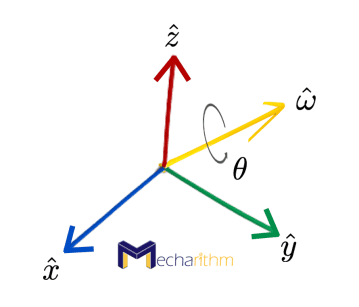
Generally, the rotation about an arbitrary unit axis ῶ

\[\hat{\omega} = (\hat{\omega}_1,\hat{\omega}_2,\hat{\omega}_3)\]

by θ can be represented by a rotation operator as:

\[Rot(\hat{\omega},\theta) = \begin{pmatrix}c_{\theta} + \hat{\omega}_1^2 (1-c_{\theta}) & \hat{\omega}_1 \hat{\omega}_2(1-c_{\theta}) -\hat{\omega}_3 s_{\theta} & \hat{\omega}_1 \hat{\omega}_3 (1-c_{\theta}) + \hat{\omega}_2 s_{\theta} \\\hat{\omega}_1 \hat{\omega}_2 (1-c_{\theta}) + \hat{\omega}_3 s_{\theta} & c_{\theta} + \hat{\omega}_2^2 (1-c_{\theta}) & \hat{\omega}_2 \hat{\omega}_3 (1-c_{\theta}) – \hat{\omega}_1 s_{\theta} \\\hat{\omega}_1 \hat{\omega}_3 (1-c_{\theta}) – \hat{\omega}_2 s_{\theta} & \hat{\omega}_2 \hat{\omega}_3 (1-c_{\theta}) + \hat{\omega}_1 s_{\theta} & c_{\theta} + \hat{\omega}_3^2 (1-c_{\theta})\end{pmatrix}\]

Where

\[s_{\theta} = sin \theta \\c_{\theta} = cos \theta\]

We will see how to derive this rotation matrix in the next lesson when talking about the exponential coordinates of rotation. For now, you can verify that it is correct by assuming ῶ = (1,0,0), (0,1,0), and (0,0,1) for rotations around x, y, and z, respectively, and get rotation matrices that we calculated above.

Visualize this rotation as the following figure:

rotation-about-arbitrary-axis — The rotation about the arbitrary axis ῶ by θ.

Note that any R ∈ SO(3) can be obtained by rotating from the identity matrix by some θ about some ῶ. Also, note that:

\[Rot(\hat{\omega}, \theta) = Rot(-\hat{\omega}, -\theta)\]

In other words, rotation about -ῶ by -θ is the same as the rotation about ῶ by θ. These are topics of the next video.

Demonstration: the Representation of the Orientation of the Elements in the Robot’s Workspace

Suppose that a camera and a gripper are attached to the end-effector of the industrial arm. The camera is used to observe the workpiece and position the end-effector in the right position, and the gripper is used to grip the workpiece. The overall system can be depicted in the figure below:

robot-arm-camera-endeffector-workpiece-rotation-matrix — A camera is attached to the robot end-effector to observe the object and position the end-effector in the right position. Four reference frames are attached to different elements in the robot’s workspace, as shown in the figure. The orientation of one frame relative to the other can be implicitly represented by a rotation matrix. This example is adapted from the first textbook by Lynch et al.

Four frames are attached to different elements in the robot’s workspace, as shown above. {a} is the frame coincident with the space frame {s}, {b} is the gripper frame, {c} is the camera frame, and {d} is the workpiece frame.

The orientation of the workpiece frame relative to the base frame can be expressed by the rotation matrix R_ad as:

\[R_{ad} = \begin{pmatrix}\hat{x}_d.\hat{x}_a & \hat{y}_d.\hat{x}_a & \hat{z}_d.\hat{x}_a \\\hat{x}_d.\hat{y}_a & \hat{y}_d.\hat{y}_a & \hat{z}_d.\hat{y}_a \\\hat{x}_d.\hat{z}_a & \hat{y}_d.\hat{z}_a & \hat{z}_d.\hat{z}_a\end{pmatrix} = \begin{pmatrix}1 & 0 & 0\\0 & 1 & 0\\0 & 0 & 1\end{pmatrix}\]

This means that the two frames have the same orientation.

The orientation of the workpiece frame relative to the camera frame can be calculated as follows:

\[R_{cd} = \begin{pmatrix}\hat{x}_d.\hat{x}_c & \hat{y}_d.\hat{x}_c & \hat{z}_d.\hat{x}_c \\\hat{x}_d.\hat{y}_c & \hat{y}_d.\hat{y}_c & \hat{z}_d.\hat{y}_c \\\hat{x}_d.\hat{z}_c & \hat{y}_d.\hat{z}_c & \hat{z}_d.\hat{z}_c\end{pmatrix} = \begin{pmatrix}0 & 1 & 0\\1 & 0 & 0\\0 & 0 & -1\end{pmatrix}\]

Now suppose we have the rotation matrix representing the orientation of the camera frame relative to the gripper frame as:

\[R_{bc} = \begin{pmatrix}1 & 0 & 0\\0 & 1 & 0\\0 & 0 & 1\end{pmatrix}\]

To calculate the orientation of the gripper frame relative to the space frame R_ab, we can use the second application of the rotation matrix to act as an operator to change the reference frame of a frame as:

\[R_{ab} = R_{ad}R_{dc}R_{cb} = R_{ad} R^T_{cd} R^T_{bc} = \begin{pmatrix}1 & 0 & 0\\0 & 1 & 0\\0 & 0 & 1\end{pmatrix} \begin{pmatrix}0 & 1 & 0\\1 & 0 & 0\\0 & 0 & -1\end{pmatrix} \begin{pmatrix}1 & 0 & 0\\0 & 1 & 0\\0 & 0 & 1\end{pmatrix} = \begin{pmatrix}0 & 1 & 0\\1 & 0 & 0\\0 & 0 & -1\end{pmatrix}\]

Note that we used the inverse of a rotation matrix equals its transpose and the subscript cancellation rule to calculate the result.

Demonstration: Successive Rotations of a Point about the Coordinate Axes of the Base Frame

Suppose p is a point in space with coordinates relative to the space frame as p_s = (5,-7,10). In the preliminaries lesson, we saw that we could represent a point in space with a vector. The point p and the corresponding vector representation can be visualized as the following figure:

point-in-space-subject-to-different-rotations-rotation-matrix-operator-1 — point P in space and the corresponding vector representation in {s} frame

Now suppose that p is rotated about the fixed-frame x-axis by 30^o, then about the fixed frame y-axis by 135^o, and finally about the fixed frame z-axis by -120^o. The rotation matrix that rotated p to the new location can be expressed as (note the order in which the rotations are written):

\[R = Rot(\hat{z},-120)Rot(\hat{y},135)Rot(\hat{x},30)\]

These rotations can easily be calculated using the rotation operators about the coordinate axes provided above.

Then the coordinates of the rotated point can be calculated as:

\[p’_s = Rp_s = \begin{pmatrix}0.3536 & 0.5732 & -0.7392\\0.6124 & -0.7392 & -0.2803\\-0.7071 & -0.3536 & -0.6124\end{pmatrix} \begin{pmatrix}5\\-7\\10\end{pmatrix} = \begin{pmatrix}-9.6364\\5.4334\\-7.1843\end{pmatrix}\]

The rotated point can be visualized as:

point-in-space-subject-to-different-rotations-rotation-matrix-operator-rotated-point — vector representation of the rotated point p after going through a rotation by 30^o about the x-axis of the base frame, then a rotation by 135^o about the y-axis of the base frame, and finally a rotation by -120^o about the z-axis of the base frame

In the next lesson, we will talk about Exponential Coordinate Representation of Rotation which is an explicit way to represent the orientation.

The video version of the current lesson can be watched at the link below:

References:
📘 Textbooks:
Modern Robotics: Mechanics, Planning, and Control by Frank Park and Kevin Lynch
A Mathematical Introduction to Robotic Manipulation by Murray, Lee, and Sastry

📃 Articles:

Cao, C.T., Do, V.P. and Lee, B.R., 2019. A novel indirect calibration approach for robot positioning error compensation based on neural network and hand-eye vision. Applied Sciences, 9(9), p.1940.

✍️ Logo design by Minro Art Group