Homogeneous Transformation Matrices to Express Configurations in Robotics
Up to this point, we have discussed orientations in robotics, and we have become familiarized with different representations to express orientations in robotics. In this lesson, we will start with configurations, and we will learn about homogeneous transformation matrices that are great tools to express configurations (both positions and orientations) in a compact matrix form.
This lesson is part of the series of lessons on foundations necessary to express robot motions. For the full comprehension of the Fundamentals of Robot Motions and the necessary tools to represent the configurations, velocities, and forces causing the motion, please read the following lessons (note that more lessons will be added in the future):
https://www.mecharithm.com/category/fundamentals-of-robotics/fundamentals-of-robot-motions/
Also, reading some lessons from the base lessons of the Fundamentals of Robotics course are deemed invaluable.
In the lesson about the degrees of freedom of a robot, we saw that in 3D physical space, we need six parameters to explicitly represent the position and orientation of a rigid body (three parameters for the position and three parameters for the orientation).
We also saw that the Configuration Space (C-space) is non-Euclidean (non-flat), and thus we need special matrices to implicitly represent that. In order to implicitly represent the configuration of a rigid body, we adopt a sixteen-dimensional 4×4 matrix subject to ten constraints (16-10 = 6). This matrix can be used to express the configuration of the body frame relative to the fixed frame.
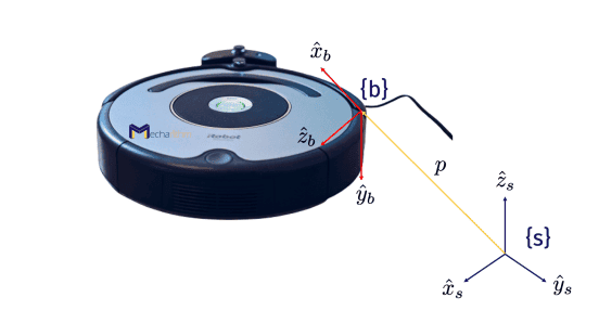
In the Introduction to Configurations lesson, we saw that the body frame is a fixed frame that is instantaneously attached to the moving body and the space frame is the fixed frame that is fixed somewhere in the space. Then the configuration of the body can be expressed by the pair (R,p) in which R ∈ SO(3) is the 3×3 rotation matrix representing the orientation of the {b} frame relative to the {s} frame and p ∈ ℝ3 is a 3-vector that is the position of the origin of the {b} frame relative to the {s} frame:
If we package both R and p into a single 4×4 matrix form, we get the homogenous transformation matrix representation of the robot’s configuration T as:
where R is a rotation matrix in the Special Orthogonal Group SO(3) and p ∈ ℝ3 is a column vector. Set of all 4×4 real matrices, T described above is called the Special Euclidean group SE(3), which is the group of rigid body motions. An element T ∈ SE(3) can also be expressed as the pair (R,p).
The advantage of adopting the 4×4 matrices to implicitly represent the configuration of a robot is the simple algebraic calculations that can be used to work with these matrices.
As many robotic mechanisms are planar:
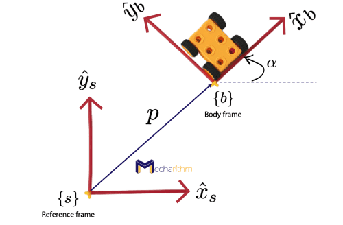
We also define another Special Euclidean Group SE(2) for planar rigid body motions. The Special Euclidean Group SE(2) is defined as the set of all 3 × 3 real matrices T of the form:
Where R ∈ SO(2), p ∈ ℝ2.
A matrix T ∈ SE(2) always has the following form:
where θ ∈ [0,2π).
For more information on how to derive the rotation matrix representing rotations in 2D, please refer to the lesson on rotation matrices.
Let’s see an example for the 2D case.
Suppose that frame {a} is instantaneously attached to a small robot and it is initillay coincident with the space frame {s}. The robot starts to move and first rotates 90o and then travels forward for five units to reach the configuration {b}, it then rotates –90o, and moves forward for five units and reaches the configuration {c} and finally it rotates –90o and moves forward for three units to reach the configuration {d}:

The homogenous transformation matrices representing the configuration of the robot at each stage can be calculated as the following:
Now let’s discuss the properties of transformation matrices.
Properties of Homogeneous Transformation Matrices to Express Configurations in Robotics
As we saw with the rotation matrices, homogenous transformation matrices have a bunch of properties that are unique to them.
- Identity matrix I is a trivial form of a transformation matrix and it means that the orientation and the origin of the body fram {b} is the same as the space frame {s}.
- The Special Euclidean Group SE(3) is a group because
(1) The inverse of a transformation matrix T ∈ SE(3) is also a transformation matrix and can be computed as
Prove this using the fact that the multiplication of a matrix with its inverse is the identity matrix and use simple matrix multiplication to find the elements of the inverse of the transformation matrix:
(2) The product of two transformation matrices is also a transformation matrix:
(3) The multiplication of transformation matrices is associative
but not generally commutative
- If we have T = (R,p) ∈ SE(3) and x,y ∈ ℝ3 then
(1) The transformation matrix T preserves distances between the points in ℝ3, which means that the distance between these points after the transformation is the same as the original distance:
in which ||.|| is the standard Euclidean norm in ℝ3
(2) The transformation matrix T preserves angles:
in which <.,.> is the standard Euclidean inner product in ℝ3
Note 1: T ∈ SE(3) as the transformation on points in ℝ3, transforms the point x to Tx and this means that the point x is rotated by R and translated by p as Rx + p; therefore Tx means the representation of x in homogenous coordinates as:
Note 2. If {x,y,z} are points on the rigid body, then {Tx,Ty,Tz} are displaced versions of the points on the rigid body.
Note 3. If x,y,z ∈ ℝ3 are three vertices of a triangle, then the triangle formed by the transformed vertices {Tx,Ty,Tz} has the same set of lengths and angles as those of the triangle {x,y,z}. These two triangles are called isometric.
Uses of Homogeneous Transformation Matrices
The homogenous transformation matrix T ∈ SE(3) can have three different applications:
(1) It can be used to express the configuration (position and orientation) of a frame relative to a fixed frame. If we consider the figure of the robot with body frame {b} and the space frame {s} that we saw at the beginning of this lesson, then the configuration of the body frame relative to the space frame can be defined as
Where Rsb is the rotation matrix representing the orientation of the frame {b} relative to the frame {s} and by now you definitely feel conformable to easily calculate it, and p is the position of the body frame {b} origin in the space frame’s coordinates.
As an illustration, suppose that three coordinate frames {a}, {b}, and {c} are positioned in space as the following figure

{a} is initially coincident with the space frame {s}. Thus, the pose of the frames {a}, {b}, and {c} relative to {s} can be calculated as
(2) It can act as an operator and change the representation of a frame or vector from one coordinate frame to another coordinate frame.
Another application for the homogenous transformation matrix is that it can act as an operator and change the reference frame of a vector or a frame. For any three reference frames {a}, {b}, and {c} and any free vector v expressed in for example {b} frame as νb then using the subscript cancellation rule that we learned before, we can write:
Here, the transformation matrix T acts as an operator and changes the reference frame of the vector or a frame. In the second equation, Tab acts on the νb and changes its reference frame from {b} to {a}. We append 1 to the end of each vector to get its homogenous coordinate representation (the 3-vector is changed into a 4-vector) and avoid dimension mismatch when applying Tab.
For example, for the example that we saw above, we can find the homogenous transformation matrix representing the pose of any frame relative to another frame. For instance, in order to calculate the homogenous transformation matrix Tbc, which represents the position and orientation of the frame {c} relative to the frame {b}, we can write:
Note that for any two frames {d} and {e} Tde = Ted-1. Using the expression for the inverse of the homogenous transformation matrix, we can calculate
And thus
Let’s see an example that uses these two applications to find the relative position and orientation of different coordinate frames.
Suppose an arm-mounted mobile robot X-Terrabot is moving in a room and wants to pick up an object with body frame {e} with its end-effector with the attached frame {c}:
A camera is fixed to the ceiling, and based on its measurements, the configuration of the frames attached to the wheeled platform {b} and the object frame {e} relative to the camera’s frame {d} are known:
Also, using the arm’s joint angle measurements, Tbc is also known:
The configuration of the camera frame {d} relative to the fixed-frame {a} is known in advance:
In order to calculate how to move the robot arm so as to pick up the object, the configuration of the object relative to the robot hand, Tce, should be determined. Using the things that we’ve learned thus far, we can write:
Therefore, the configuration of the object relative to the robot’s end-effector can be calculated as:
Now, let’s see another example. In this example, we go back to an example from the lesson about rotation matrices, and this time we are not solely interested in the orientation, but we want to calculate configurations.
Suppose that a camera and a gripper are attached to the end-effector of the industrial arm. The camera is used to observe the workpiece and position the end-effector in the right position, and the gripper is used to grip the workpiece. The overall system can be depicted in the figure below:

Four frames are attached to different elements in the robot’s workspace, as shown above. {a} is the frame coincident with the space frame {s}, {b} is the gripper frame, {c} is the camera frame, and {d} is the workpiece frame.
First, we want to calculate the configuration of the workpiece frame {d} relative to the frame {a} and the camera frame {c}. To this end, we just need to calculate the homogenous transformation matrices, Tad and Tcd. In the lesson about the rotation matrices, we calculated the orientation part of the transformation matrix. Now, we just build up the configuration matrix with the position data as:
Now, suppose that the configuration of the camera frame {c} relative to the end-effector frame {b} is given as:
And we’d like to calculate the configuration of the end-effector frame {b} relative to the frame {a}. To this end, we use the subscript cancellation rule, and we can write:
(3) It can act as an operator and can be used to translate and rotate (displace) a frame or a vector.
The homogenous transformation matrix can act on a vector or a frame and displaces (rotating and translating) it. Then T = (R,p) can be expressed as T = (Rot(ῶ,θ),p) and can act on a vector or a frame and rotate it by θ about an axis ῶ and translate it by p.
By abuse of notation, we can define the 3×3 rotation operator R = Rot(ῶ,θ) as a 4×4 transformation matrix that rotates but not translates as
And the 4×4 transformation matrix that can act as the translation operator and can only translate but cannot rotate can be defined as
This translation operator causes a translation along the unit direction p̂ by a distance ||p||.
Now let’s see the effect of pre-multiplying or post-multiplying a transformation matrix by the operator T = (R,p). Suppose that Tsb is the configuration of the body frame {b} relative to the space frame {s} and T = (Rot(ῶ,θ),Trans(p)) is the rotation and translation operator. Then we have two cases
(1) Fixed-frame transformation: if we pre-multiply Tsb by T, then ῶ, and p are interpreted in the space frame {s}:
In this case, the operator T = (Rot(ῶ,θ),Trans(p)) first rotates the body frame {b} by θ about an axis ῶ in the space frame {s} and then translates it by p in the space frame {s} to get {b’}. If the origin of the body frame {b} is not coincident with the origin of the space frame {s}, then the rotation moves the origin of the body frame {b}.
(2) Body-frame transformation: if we post-multiply Tsb by the operator T, then the rotation axis ῶ and the position vector p are both interpreted in the body frame {b}:
In this case, the operator T = (Rot(ῶ,θ),Trans(p)) first translates the body frame {b} by p considered to be in the body frame {b}, then rotates about ῶ in the new body frame by θ to get the new frame {b”}. This rotation does not move the origin of the frame.
Let’s see all these with examples.
Suppose that the configuration of the body frame {b} relative to the space frame {s} is as the following figure:
Where the configuration of the body frame relative to the space frame, as we saw earlier in the lesson, can be represented by a 4×4 transformation matrix as
Now suppose that displacement (rotation and translation) operator T = (Rot(ῶ,θ),Trans(p)) corresponds to a rotation about the unit axis ῶ = (0,0,1) by θ = 90o and a translation along the vector p = (0,2,0). Let’s find the final pose (position and orientation) of the body frame relative to the space frame after going through a transformation of pre-multiplying or post-multiplying of the transformation matrix representing the configuration of the body frame relative to the space frame by the displacement operator defined.
Case (1): Tsb is pre-multiplied by T, then the rotation axis ῶ is interpreted in the space frame {s} and is equal to the axis ẑs. p is also interpreted in the {s} frame and represents a translation of two units along the ŷs axis. Then the final pose of the body frame relative to the space frame can be visualized as
The frame {b} first goes through a rotation by 90o about the z-axis of the {s} frame, and because the origins of the frames {b} and {s} are not initially coincident, this rotation displaces the origin of the {b} frame. Then it goes through a translation by two units along the y-axis of the space frame {s} to reach the frame {b’}. The simulation below shows a demonstration of this transformation:
Mathematically, we can say that the transformation matrix representing the pose of the frame {b’} relative to the space frame {s} can be calculated as
where Rot(ῶ,θ) can be calculated using the Rodrigues’ formula that we learned in the lesson about the exponential coordinate representation of orientation as
And then, we wrote it as a 4×4 rotation operator.
This result can also be verified from the figure.
Case (2): Tsb is post-multiplied by T (body-frame transformation), then the rotation axis ῶ and the position vector p are both interpreted in the body frame {b}. In this case, first, a translation along the {b} frame’s y-axis, ŷb, is done by two units, and then a rotation about the new body frame’s z-axis is done by 90o. This rotation does not change the origin of the new body frame. The final pose of the body frame relative to the space frame can be visualized as
The simulation below shows a demonstration of this transformation:
Mathematically, we can also prove this. The transformation matrix representing the pose of the frame {b”} relative to the space frame {s} can be calculated as
That verifies the result that we got from the visualization.
That’s going to wrap up today’s lesson. We hope that it gave you a good understanding of homogenous transformation matrices and their applications. The next lesson is about the Exponential Coordinate Representation of Robot Motions. Stay Tuned! See you in the next lesson!
The video version of the current lesson can be watched at the link below:
References:
📘 Textbooks:
Modern Robotics: Mechanics, Planning, and Control by Frank Park and Kevin Lynch
A Mathematical Introduction to Robotic Manipulation by Murray, Lee, and Sastry
📃 Articles:
- Cao, C.T., Do, V.P. and Lee, B.R., 2019. A novel indirect calibration approach for robot positioning error compensation based on neural network and hand-eye vision. Applied Sciences, 9(9), p.1940.