Screws: a Geometric Description of Twists in Robotics
In the previous lesson, we learned about velocities in robotics. We became familiar with angular and linear velocities and saw that stacking them together gives us the twist. We also saw how we could change the frame of reference for angular velocities and twists.
This lesson is about screws as a geometric interpretation for twists and how they can be used to express configurations in robotics.
This lesson is part of the series of lessons on foundations necessary to express robot motions. For the complete comprehension of the Fundamentals of Robot Motions and the tools required to represent the configurations, velocities, and forces causing the motion, please read the following lessons (note that more lessons will be added in the future):
Also, reading some lessons from the base lessons of the Fundamentals of Robotics course are deemed invaluable.
Ok, now let’s see how twists and screws are related.
In a couple of lessons before, we saw that every rigid body displacement could be obtained by a finite rotation about and translation along a fixed screw axis 𝘚 and we became familiar with the exponential coordinates of robot motions. We saw that in order for us to define the screw axis, we needed to learn about velocities, and now that we have the necessary foundation for it, we can go back and look at the screw motion again. These tools will equip us for the robot kinematics lesson in the near future.
In the Velocities in Robotics lesson, we learned that the angular velocity ω could be represented by a unit axis ω̂ and the rate of rotation θ̇ about this axis. Similarly, we can express a twist (that has an angular component and a linear component) as a screw axis 𝘚 and the rate θ̇ about this axis:
Any robot configuration can be achieved by starting from the home (fixed) reference frame at time t = 0 (T(0) = I) and then integrating this twist over a specified time to reach the final configuration, as we also saw before.
On the other hand, any rigid body velocity has a linear component and an angular component equivalent to the instantaneous velocity about some screw axis.
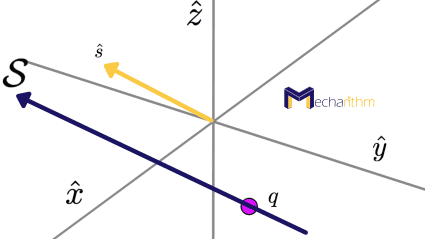
Suppose that the configuration of the body frame relative to the space frame at any time is represented by a rotation about and translation along the screw axis 𝘚 with the rate θ̇ (a scalar that shows how fast the body moves along the screw). The figure below shows this representation:
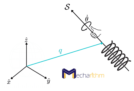
The screw axis 𝘚 can be represented in two ways.
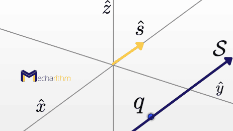
{q,ŝ,h} Interpretation of the Screw Axis
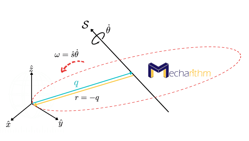
First, the screw axis can be represented by any point on the axis q ∈ ℝ3, the unit vector in the direction of the screw axis ŝ, and the screw pitch h, which is the linear speed along the screw axis divided by the angular speed θ̇ about the screw axis: {q,ŝ,h}.
The twist about the screw axis 𝘚 represented by {q,ŝ,h} can be defined as:
ω is the angular velocity, and it is in the direction of the unit vector ŝ with the magnitude θ̇, and the linear velocity v has two parts. hŝθ̇ is due to translation along the screw axis (in the ŝ direction) that exists when the screw has non-zero pitch and ω×r = ŝθ̇×(-q) = -ŝθ̇×q is due to the linear motion at the origin which is the result of the rotation about the screw axis. We saw before that the linear velocity during the circular motion (that has zero pitch = no translational motion) is tangential to the circular path, and it can be calculated by the cross product of the angular velocity and the radius of the path (this is in the plane orthogonal to ŝ):
Now think in the reverse fashion. If we have the twist 𝒱 = (ω,ν) and we want to find the screw axis {q,ŝ,h} and θ̇ that can generate the same twist, we will have two cases.
Case one is where we have rotational motion (ω ≠ 0), and the screw pitch is finite. If the angular velocity is not zero (we also have rotational motion), then the pitch h is finite, and θ̇ is the norm of the angular velocity vector (θ̇ = ||ω||). Then because ω = ŝθ̇ = ŝ||ω||, we can find ŝ = ω/||ω|| = ω̂. The pitch can be calculated using the equation h = ω̂Tν/||ω|| and q is chosen so that the term -ŝθ̇×q provides the portion of ν orthogonal to the screw axis.
Case two is where there is no rotational motion (ω = 0), and thus the pitch h is infinite and ŝ = ν/||ν|| and θ̇ is the linear speed ||ν|| along ŝ.
In this representation of the screw axis 𝘚, the pitch can be infinite, q is not unique (any point along the screw axis can be used), and it is a cumbersome collection. Hence, we opt for an alternative representation for the screw axis 𝘚.
Screw Interpretation of a Twist in Robotics
As an alternative representation, the screw axis 𝘚 is defined as follows. First, we choose a reference frame and then define the screw axis 𝘚 as the 6-vector in that frame’s coordinates as:
𝘚ω is the 3D unit angular velocity when the rate θ̇ = 1 and 𝘚ν is the 3D linear velocity of the origin of the frame when the rate is 1. We can conclude that the screw axis is a normalized twist and thus, the twist 𝒱 = (ω,ν) can be represented by the multiplication of the screw axis 𝘚 by the scalar rate θ̇ (𝘚θ̇). In this case, as we discussed, the screw axis 𝘚 can be defined using a normalized version of the twist 𝒱 = (ω,ν) corresponding to motion along the screw.
As before, we will have two cases:
Case one is when there is a rotational component and ω≠0, and therefore the pitch h is finite. The angular component 𝘚ω of the screw axis is nonzero and the twist, 𝒱 is normalized by the norm of the angular velocity vector:
θ̇ = ||ω|| is the angular speed about the screw axis such that 𝘚 θ̇ = 𝒱. ||𝘚ω|| = 1 because we normalized it with the angular speed. 𝘚ν is arbitrary, with no constraints on it.
Case two is when there is no rotational motion (ω=0), and thus the pitch h is infinite. In this case, the motion is a purely linear motion with no rotation. The angular component is zero, and the linear part is a unit vector. In this case, the twist, 𝒱 is normalized by the length of the linear velocity vector:
θ̇ = ||ν|| is the linear speed along the screw axis such that 𝘚 θ̇ = 𝒱. For this case, 𝘚ω = 0, ||𝘚ν|| = 1 since we normalized it.
Note here that six numbers are needed to represent the screw axis 𝘚 = (𝘚ω,𝘚ν), but the space of all screws is five-dimensional (5D), and this is because either 𝘚ω or 𝘚v has a unit length. As discussed, if both the angular and linear components of the screw are non-zero meaning that we have a rotational motion as well, then the screw is defined so that ||𝘚ω|| = 1.
Now let’s see how we can define the matrix representation of the screw axis 𝘚.
Matrix Representation of the Screw Axis 𝘚
Since the screw axis is the normalized version of the twist, then the matrix representation of the screw axis 𝘚 = (𝘚ω,𝘚v) can be defined as (for more information on why it has this matrix form, please refer to the lesson on the velocities in robotics):
Now let’s see how we can change the frame of reference in which a screw axis 𝘚 is defined.
Change of Frame of Reference of a Screw Axis 𝘚
As we saw in the lesson on the velocities in robotics, the adjoint transformation could be used to change the frame of reference of the twist, and since the screw axis is a normalized twist, we can use the adjoint transformation to change the frame of reference of the screw axis as well:
𝘚a is the screw axis representation in the frame {a}, and 𝘚b is the screw axis representation in the frame {b}.
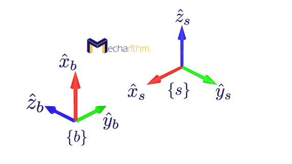
If the screw axis 𝘚 is expressed in coordinates of the body frame {b}, 𝘚b, then 𝒱b = (ωb,νb) = 𝘚bθ̇ is called the body twist which is not affected by choice of the space frame, and if the screw axis 𝘚 is expressed in coordinates of the space frame {s}, 𝘚s, then 𝒱s= (ωs,νs) = 𝘚sθ̇ is called the spatial twist which is not affected by choice of the body frame. Thus, we only need to define the frame in which the twist (or screw) is represented. No other frames matter. A spatial twist depends on the {s} frame, and a body twist depends on the {b} frame.
Now, based on our knowledge about the screw axis, let’s go back to the exponential coordinate representation of rigid body motions.
Exponential Coordinate Representation of Rigid Body Motions
In the exponential coordinate representation, 𝘚θ ∈ ℝ6:
- If pitch of the screw axis 𝘚 = (𝘚ω,𝘚v) is finite then we have rotational motion and θ is the angle of rotation about the screw axis.
- If the pitch is infinite then the motion is pure translation with no rotation and θ is the linear distance travelled along the screw axis.
As we saw in the lesson about the exponential coordinates of rotation, the matrix exponential e[ω̂]θ is equal to the rotation matrix that can act on a vector or a frame and can rotate it from the initial orientation to the final orientation. Similarly, the matrix representation of the screw axis can be used in the matrix exponential e[𝘚]θ for rigid body motions. Thus, the matrix exponential for rigid body motions can map the elements of the Lie algebra se(3) to the elements of the Lie group SE(3):
exp: [𝘚]θ ∈ se(3) → T ∈ SE(3)
And this means that exponentiation takes the initial configuration of the frame to the final configuration of the frame by following along and about a screw axis 𝘚 by θ.
And the matrix logarithm is the invert of the matrix exponential and finds the matrix representation of the exponential coordinates 𝘚θ:
log: T ∈ SE(3) → [𝘚]θ ∈ se(3)
And this means that if we have a given configuration, we want to find the screw axis and θ such that if followed along and about this screw axis by that amount gives the same configuration.
The normalized (unit) screw axis for full spatial motions is similar to the normalized angular velocity axis for pure rotations.
As we found a closed-form solution for the matrix exponential e[ω̂]θ for orientations before, let’s examine if we can do the same for the matrix exponential e[𝘚]θ for rigid body motions. Let the screw axis be 𝘚 = (𝘚ω,𝘚ν) then we will have two cases:
- If we have rotational motion, then for any distance θ ∈ ℝtravelled along the axis, the matrix exponential for rigid body motions can be written as:
- And if the rotational part is zero and the screw axis is pure translation with no rotation, then:
Here, θ is the linear distance traveled. The matrix I in the upper left of the matrix shows that the orientation does not change, and the motion is pure translation.
The proof is similar to the approach that we used in the lesson about the exponential coordinates of rotation for the matrix exponential.
The inverse problem says that given an arbitrary configuration (R,p) ∈ SE(3), we can always find a screw axis 𝘚 = (𝘚ω,𝘚ν) and a scalar θ such that
And as we saw before, the matrix
is called the matrix logarithm of T = (R,p).
To solve the inverse problem, we follow the following algorithm:
Given (R,p) written as T ∈ SE(3), find a θ ∈ [0,π] and a screw axis 𝘚 = (𝘚ω,𝘚ν) ∈ ℝsuch that e[𝘚]θ = T. The vector 𝘚θ ∈ ℝ6 comprises the exponential coordinates for T, and the matrix [𝘚]θ ∈ se(3) is the matrix logarithm of T.
(a) If R = I then set 𝘚ω = 0 and 𝘚ν = p/||p|| and θ = ||p||.
(b) Otherwise, use the matrix logarithm on SO(3) that we learned in the exponential coordinates for rotations lesson to determine 𝘚ω (= ω̂ ) and θ for R. The 𝘚ν is calculated as 𝘚ν = G-1(θ)p where G-1(θ) = 1/θ I – 1/2[𝘚ω] + (1/θ – 1/2 cotθ/2)[𝘚ω]2.
Note that every single-degree-of-freedom joint (revolute joint, a prismatic joint, and a helical joint) of a robot that we talked about in the degrees of freedom lesson has a joint axis defined by a screw axis, and thus, we can conclude that the matrix exponential and the logarithm can be used to study the robot kinematics as we will see in the coming lessons:
Now let’s see some examples that use all the knowledge that we have learned thus far to find solutions.
Example: Homogenous Transformation Matrix to Exponential Coordinates of Motion
Suppose that the configuration of the body frame relative to the space frame is as the following figure:
In which the origin of the {b} frame is at (3,0,0) in terms of the space frame coordinates. The configuration of the {b} frame relative to the {s} frame, as we learned in the lesson about the homogenous transformation matrices, can be found using the transformation matrix Tsb as:
We want to find the screw motion (the screw axis 𝘚 and the amount of traveled distance θ about the screw axis) that can generate the same configuration.
Since the orientation of the body frame is not the same as the orientation of the space frame, then we have a rotational motion. Using the approach we learned in the lesson about the exponential coordinates of orientation for the matrix logarithm of rotations, we can easily find the unit axis and the amount of rotation about this axis that can produce the given orientation as:
So, a rotation of 120o about the unit axis calculated above will create the same orientation. Now, using the second approach to calculate the screw axis, we can say that the
And
And thus the screw axis can be defined as:
Therefore, a screw motion about the screw axis 𝘚 calculated above with the amount of θ calculated earlier produces the same configuration defined by the homogenous transformation matrix Tsb.
For more practice, let’s find the {q,ŝ,h} representation of the screw axis and draw it. Since we have rotational motion, then we use the equations for the first case and can calculate the screw axis parameters as:
Note that q is not unique and the calculated q is only one feasible answer that can be calculated solving the equation v = -ŝθ̇×q + hŝθ̇. Therefore, the screw axis can be visualized as:
Now let’s see another example.
Example: Screw Motion Corresponding to a Given Twist
We want to find and visualize the screw axis which if followed at a specific rate will correspond to the given twist 𝒱 = (0,2,2,4,0,0).
From the screw representation of a twist, we can write:
Since the rotational part is not zero, we also have rotational motion and we should normalize the twist using the norm of the angular velocity:
Therefore, it is easy to see that the rate θ̇ = 2.828 and the screw axis is equal to:
Therefore the {q,ŝ,h} representation of the screw axis can easily be calculated as:
And therefore, the screw axis can be visualized as:
Since the screw pitch is zero, the motion is pure rotation with no translational motion about the screw axis. Therefore, a screw motion about the above screw axis by the rate of θ̇ calculated above can produce the given twist (𝘚θ̇).
Example: Exponential Coordinates of Motion to Homogenous Transformation Matrix
In this example, we want to go backward and find the homogenous transformation matrix corresponding to the given exponential coordinates of the motion.
Suppose that the exponential coordinates of the motion are given by the following matrix:
In order to find the homogenous transformation matrix representing the same configuration, we should find the matrix exponential corresponding to the exponential coordinates. Since the upper matrix part is not zero, we have rotational motion and thus the rotational part of the screw axis should be normalized. Thus we can write:
From the screw axis that we calculated, it will be easy to calculate the matrix exponential of the motion through the following process:
And using the Rodrigues’ formula that we learned in the lesson about the exponential coordinates of orientation, we can find the rotational part of the transformation matrix as:
And the linear part can be calculated as
Therefore the homogenous transformation matrix representing the same configuration can be calculated as:
This homogenous transformation matrix represents the same configuration as the configuration of the frame after going through a screw motion about the defined screw axis. The initial configuration is the identity matrix since the {b} frame is initially coincident with the frame {s}.
Now let’s see how we can find the body frame’s final configuration after traveling a distance θ along the screw axis 𝘚 if the screw axis is defined in the space or the body frame.
Body Frame’s Final Configuration After Travelling along the Screw Axis Defined in the Space or the Body Frame
Suppose that the space frame {s} and the body frame {b} are configured in space as the following figure:
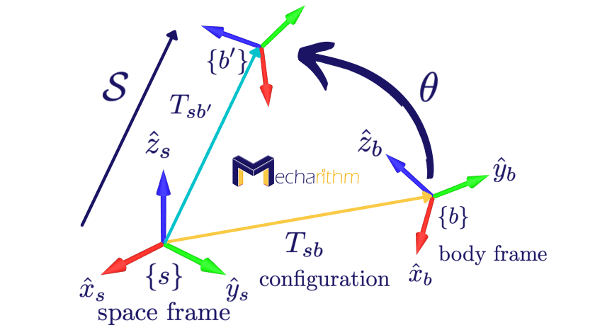
The configuration of the body frame relative to the space frame can be found using the matrix Tsb. We would like to know the body frame’s final configuration, Tsb’ if it travels a distance θ along the screw axis 𝘚. We would have two cases since 𝘚 can be represented in either {b} or {s} frame.
- If the screw axis 𝘚 is expressed in the {b} frame then the final configuration of the body frame can be calculated using the equation Tsb’ = Tsb e[𝘚b]θ. In this case, the transformation matrix representation of the {b} frame relative to the {s} frame, Tsb, is post-multiplied by the matrix exponential.
- If the screw axis 𝘚 is expressed in the {s} frame then the final configuration of the body frame can be calculated using the equation Tsb’ = e[𝘚s]θ Tsb. In this case, the transformation matrix representation of the {b} frame relative to the {s} frame, Tsb, is pre-multiplied by the matrix exponential.
That’s going to wrap up today’s lesson. We hope that it gave you a good understanding of screws in robotics. In the next lesson, we will talk about forces in robotics. Stay Tuned! See you in the next lesson!
The video version of the current lesson can be watched at the link below:
Thanks for reading this post. You can also find the other posts on the Fundamentals of Robotics Course in the link below.
References:
Textbooks:
Modern Robotics: Mechanics, Planning, and Control by Frank Park and Kevin Lynch
A Mathematical Introduction to Robotic Manipulation by Murray, Lee, and Sastry