Velocities in Robotics: Angular Velocities & Twists
In the previous lesson, we saw an introduction to screw theory and its applications in robotics. We saw that integrating a constant twist over time gives us the configuration. We also became familiar with the exponential coordinates of robot motions, and we saw that in order to define the screw axis, we need to understand angular and linear velocities.
In this lesson, we will become familiar with the concept of velocities in robotics, and we will study angular velocities and twists. This lesson is part of the series of lessons on foundations necessary to express robot motions. For the complete comprehension of the Fundamentals of Robot Motions and the tools required to represent the configurations, velocities, and forces causing the motion, please read the following lessons (note that more lessons will be added in the future):
Also, reading some lessons from the base lessons from the Fundamentals of Robotics course are deemed invaluable.
A rigid body’s velocity can be represented as a point in a 6D space, consisting of the angular velocity and the linear velocity, which together is called a spatial velocity or a twist. From this, we can conclude that although a robot’s C-space is not Euclidean (refer to the lesson on the C-space of the robot) and thus non-flat and does not form a vector space, the space of the robot velocities always forms a vector space (a plane tangent to the robot’s C-space at any point on the C-space).
There are several ways to express the angular velocities and twists that we will discuss in the coming paragraphs.
Angular Velocities in Robotics
Unlike the space of orientations that is curved and cannot globally be expressed by three numbers without singularities, space of angular velocities is a flat 3D space (or a linear vector space) tangent to the curved 3D surface of orientations at any given orientation, and thus the 3D velocity space can be explicitly parameterized by three numbers without singularities. If we take the curved space of orientations SO(3) as a sphere, then the space of angular velocities is a flat 3D vector space tangent to SO(3) at that orientation:

Note that the 3D vector space can be represented globally by three coordinates without any singularities.
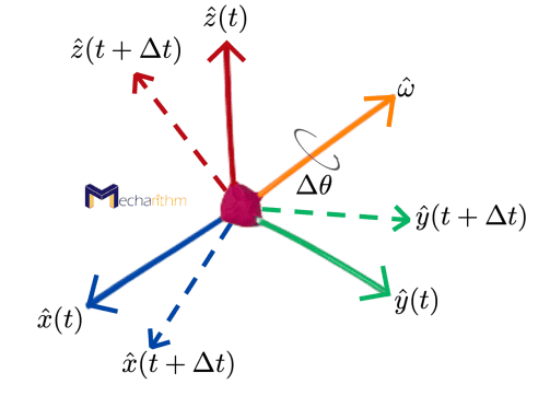
In order to understand the angular velocity concept, suppose a rotating body with the coordinate frame axes attached to it at time t and rotating with the body about an arbitrary axis passing through the origin by an angle Δθ. The axis of rotation is coordinate-free for now, which means that it is not yet represented in any particular frame.
A small change in the orientation of this frame can be depicted as the figure below (note that each of the coordinate axes is of unit length, so only the direction can vary with time):
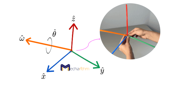
Video below shows the visualization of the rotation of the coordinate frame instantaneously attached to a rotating body about an arbitrary axis in space:
The rate of rotation of the moving body about the arbitrary axis can be defined as:
Note that the rate of rotation is analogous to the concept of speed in physics, which is a number compared to the velocity that has an amplitude and a direction.
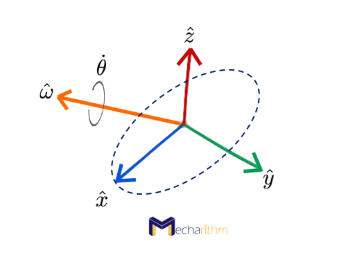
Therefore the rotation of a rotating body about an arbitrary axis with a known speed (rate) of rotation can be visualized as the following figure:
The motion of the frame as it rotates about the arbitrary axis is according to the right-hand rule, and any angular velocity can be represented by a rotation axis and the speed of rotation about it:
As the coordinate axes rotate about the arbitrary axis, the coordinate axes trace a circular path, as we saw in the video. For instance, if the coordinate frame axes shown in the figure below rotate with a constant rotational speed about the arbitrary axis, each of the coordinate axes traces a circular path as it is shown for the x-axis:
From physics, we know that an object in circular motion experiences a centripetal acceleration, and the linear velocity is in the direction tangent to the circle that can be calculated from the cross product of the angular velocity and the radius vector (we also saw this in the example of the salad spinner in the lesson about the exponential coordinates of orientations). Similarly, here, the linear velocity of each axis is in the direction tangent to the circle, and it is the cross product of the angular velocity and the radius vector, which is the axis itself. For example for the x-axis, it is like this:
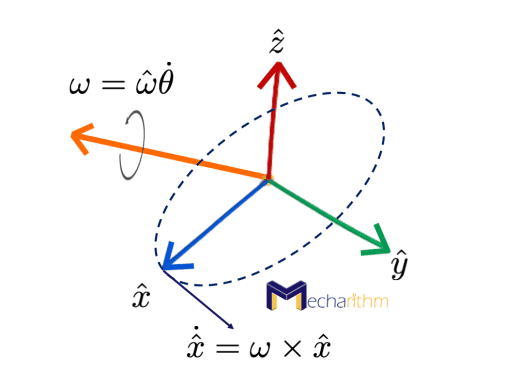
So the linear velocities of frame axes rotating about an arbitrary axis with a known angular velocity are in the direction tangent to the circular path and can be calculated as:
Now let’s see how we can define the angular velocity with respect to different coordinate frames.
Expressing the Angular Velocity Relative to Different Coordinate Frames
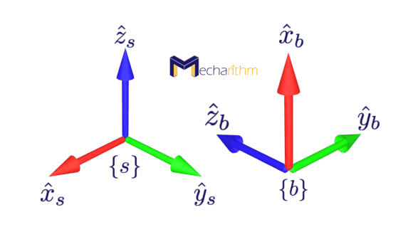
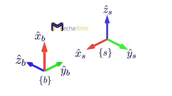
Now we want to express the above equations with respect to coordinate frames. We can choose a reference frame for the angular velocity, and our natural choices are the fixed frame {s} and the body frame {b}. If the rotation axis is defined in the {s} frame, then the angular velocity expressed in the {s} frame can be written as:
A similar equation can be written for the angular velocity expressed in the {b} frame. We then want to find expressions for the angular velocities in the {s} and {b} frames in terms of the rotation matrix. Suppose that R(t) is a rotation matrix that represents the orientation of the body frame with respect to the fixed frame at time t that can be expressed in terms of its column vectors as:
As we know from the rotation matrices lesson, the column vectors of this rotation matrix are the coordinate axes of the body frame expressed in the fixed frame coordinates. Thus the time rate of change of R(t) can be described as:
Where [ωs] is the 3×3 skew-symmetric matrix representation of the angular velocity ωs ∈ ℝ3 expressed in the fixed frame coordinates at a specific time. As we saw in the exponential coordinates of the orientation lesson, we use this notation to eliminate the cross-product.
Also, in the same lesson, we defined the set of all 3×3 real skew-symmetric matrices as so(3), which is the Lie algebra of the Lie group SO(3) that we defined in the lesson about rotation matrices. In other words, so(3) consists of all possible Ṙ when R = I:
With the above definition, we can now write the angular velocity vector in {s} frame as:
From the rotation matrices lesson, we know that the inverse of a rotation matrix is the same as its transpose: R-1 = RT.
Now we want to find the angular velocity vector in the body frame coordinates. Note that ωs and ωb are two different representations of the same angular velocity ω. In the lesson about rotation matrices, we learned that one of the applications of a rotation matrix is to serve as an operator to change the frame of reference of a frame or a vector. Thus we can find the relationship between the two different representations of the angular velocity using the rotation matrix and the subscript cancellation rule:
Therefore,
Now we want to write the skew-symmetric matrix form of the angular velocity vector in the body frame:
This equation is derived using the fact that for any angular velocity ω ∈ ℝ3 and rotation matrix R ∈ SO(3), we can write:
Proof: Suppose that we define the rotation matrix R in terms of its row vectors as:
Then,
Here, we should use the determinant formula for 3×3 matrices. Suppose that A is a 3×3 matrix with columns {a1,a2,a3}, then
Therefore,
Note we used the fact that r1, r2, and r3 are coordinate axes, and they follow the right-hand rule:
We also used the two properties of the cross product as follows:
The cross product of one axis with itself is zero (since the sine of the angle between two vectors is zero):
and the cross product of rj and ri is in the opposite direction of the cross product of ri and rj
In summary, equations relating R (orientation of the rotating frame as seen from the fixed frame) and Ṙ to the angular velocity of the rotating frame ω can be written as follows:
Where ωb ∈ ℝ3 is the body frame vector representation of ω and [ωb] ∈ so(3) is its 3×3 skew-symmetric matrix representation. Similarly, ωs ∈ ℝ3 is the fixed frame representation of ω and [ωs] ∈ so(3) is its 3×3 matrix representation.
Note that ωb is not the angular velocity relative to a moving frame, but rather it is the angular velocity relative to the stationary frame {b} instantaneously coincident with a frame attached to the moving body. This is from Newton’s laws that the reference frames are always considered to be inertial.
Also, note that fixed-frame angular velocity ωs is not dependent on the choice of the body frame, and the body-frame angular velocity ωb is not dependent on the choice of the fixed frame. This is because although R and Ṙ are individually dependent on both the {s} and {b} frames, the product ṘR-1 is independent of the {b} frame, and the product R-1Ṙ is independent of the {s} frame.
Note also that we can represent the angular velocity expressed in an arbitrary frame {d} in another frame {c} if we know the rotation that takes the {c} to {d}:
To conclude this section, let’s see some examples.
Example 1:
Consider that the Pepper robot from SoftBank Robotics is rotating its elbow while keeping all other joints fixed:
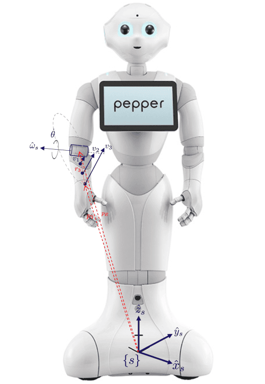
Then the linear velocities of the points on the forearm satisfy the following equations:
Note that the points farthest from the center of the elbow have larger linear velocities. The radius of rotation is measured from the center of rotation to the point.
Example 2:
Suppose that in terms of the axes of the space frame {s}, the body frame’s x-axis and y-axis are in (0,0,1) and (-1,0,0) directions, respectively. An angular velocity ω is expressed in the {s} frame as ωs = (3,2,1). We want to find the representation of the angular velocity in {b} frame coordinates.
For this, the two frames {s} and {b} can be drawn as
Note that since we do not have the position information, we can suppose that the origins are the same, and they are illustrated separately for clarification.
As we just learned, we can represent the angular velocity in another coordinate frame using the rotation matrix representation of the orientation of one frame relative to the other. For our example, we can write:
The rotation matrix representing the orientation of the {s} frame relative to the {b} frame can be calculated by taking the transpose of the rotation matrix representing the orientation of the {b} frame relative to the {s} frame as:
Thus the representation of the angular velocity in the body frame can be calculated as:
Now, let’s see what the concept of twists means in Robotics.
Twists in Robotics
In the previous lesson, we saw that integrating a constant twist over time gives us the configuration. We now want to argue that a twist is, in fact, continuous change in pose over time.
A twist can be defined as an angular velocity and the linear velocity of a moving body combined together into a compact 6-vector:
In the section about the angular velocities, we saw that pre- or post-multiplying Ṙ by R-1 results in the skew-symmetric matrix representation of the angular velocity vector either in the fixed- or the body-frame coordinates. Let’s find out if similar physical interpretations hold for the multiplications T-1Ṫ and ṪT-1.
Suppose that {s} is the fixed (space) frame and {b} is the moving (body) frame:
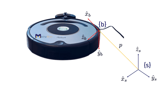
and the configuration of the body frame {b} as seen from the space frame {s} is defined as:
Then we can write:
Refer to the lesson on homogenous transformation matrices to understand how to calculate the inverse of the transformation matrix T. As we saw in the angular velocities section, RTṘ is the skew-symmetric matrix representation of the angular velocity in {b} coordinates, [ωb]. ṗ is the linear velocity of the origin of the {b} frame expressed in the fixed frame {s}, and thus RTṗ is the linear velocity of the origin of the {b} frame defined in the {b} frame:
This makes sense since RTsb = R-1sb = Rbs and the multiplication of Rbs and ṗs changes the reference frame from {s} to {b} (subscript cancellation rule). For more information, please refer to the lesson about the rotation matrices and study their different applications.
Therefore, T-1Ṫ can be re-written in terms of the angular velocity and the linear velocity as:
Where [ωb] ∈ so(3) and νb ∈ ℝ3. Thus we can conclude that T-1Ṫ represents the linear and angular velocities of the moving frame relative to the stationary frame {b} currently aligned with the moving frame and more accurately, it represents the matrix representation of the body twist, which is the spatial velocity in the body frame and can be defined as:
Note that here bracket notation [] shows the matrix representation of the body twist. It’s important to distinguish between [ω] and [𝒱]. In [ω], the bracket notation means the skew-symmetric matrix representation of an angular velocity, whereas, in [𝒱], the bracket notation refers to the matrix representation of a twist.
T-1Ṫ is the matrix representation of the body twist defined above that belongs to se(3), which is the set of all 4×4 matrices of this form. se(3) is the matrix representation of the twist associated with the rigid body configuration in SE(3). In other words, se(3) is the Lie algebra of the Lie group SE(3) and consists of all possible Ṫ when T = I. In other words, the set of all 4×4 real matrices with a 3×3 so(3) matrix at the top left, and four zeros in the bottom row is called se(3), which is the space of 4×4 matrix representation of twists. The top left 3×3 submatrix, as we discussed, is the skew-symmetric matrix representation of the angular velocity. The top right is a 3×1 vector which is the linear velocity of a point at the origin of the body frame expressed in that frame.
We will use these matrix representations for the matrix exponential and logarithm for rigid body motions in the next lesson, as we did for the matrix exponential and logarithm for rotations.
We can find a similar physical interpretation for the multiplication ṪT-1 as:
In the angular velocity section, we saw that ṘRT is the skew-symmetric matrix representation of the angular velocity expressed in the fixed frame coordinates. Now let’s figure out what vs = ṗ – ṘRTp= ṗ – [ωs]p = ṗ – ωs×p means which is obviously not the linear velocity of the body frame origin expressed in the fixed frame (which we know that equals to ṗ). Suppose we have an infinitely large rigid body that the origins of the frames {s} and {b} are two points on this rigid body, and p is the location of the origin of the {b} frame relative to the {s} frame:
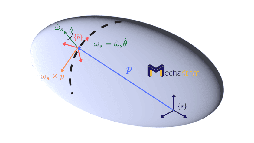
As the body moves, the origin of the {b} frame traces a circular path of radius p relative to the origin of the frame {s}. From the dynamics of rigid bodies, we can easily write the motion of the origin of the frame {b} relative to the motion of the origin of the frame {s} as:
Where ωs = ω̂sθ̇ is the angular velocity of the rigid body expressed in the frame {s}; therefore ωs × p is the linear velocity of the origin of the frame {b} during rotational motion that is tangent to the circular path expressed in the {s} frame. Therefore, we can conclude that vs is the instantaneous velocity of the point on the infinitely large rigid body currently at the origin of the {s} frame expressed in the {s} frame. With these definitions, the spatial twist, which is the spatial velocity in the space frame, can be expressed as:
And the matrix representation of the spatial twist can be found as:
Note that here, as we discussed earlier, the bracket notation does not imply a skew-symmetric matrix, but it only wants to show the 4×4 matrix representation of the twist.
Also, note that like the angular velocity, for any given twist, its fixed-frame representation 𝒱s is not dependent on the choice of the body frame, and its body frame representation 𝒱b does not depend on the choice of the fixed frame.
From the equations that we obtained for the body twist and the spatial twist, we can find a relationship between them. The matrix representations of the body twist and the spatial twist will then have the following relationship:
Expanding one of the equations and inserting the values for T and T-1, we can find a relationship between the spatial and the body twists:
We saw that R[ω]RT = [Rω] and it is easy to see that [ω]p = -[p]ω for p,ω ∈ ℝ3 ([ω]p = ω×p = -p×w = -[p]ω ). Inserting these into the above equation, we get the following relationship for the matrix representation of the spatial twist:
Therefore, we can write the relationship between the spatial twist and the body twist as:
This relationship is beneficial when changing the frame of reference for twists and wrenches that we will study in the next lesson.
Similarly, we can find a similar relationship for the body twist in terms of the spatial twist:
Therefore,
Note that both the body twist and the spatial twist represent the same motion just in different coordinate frames.
The matrix that can change the frame of representation of a twist or a screw is called the Adjoint representation of a transformation matrix Tab. The adjoint and not the transformation matrix T is used to change the frame of representation of a twist because of dimension mismatch. 𝒱a = [AdTab] 𝒱b is the modified version of the subscript cancellation rule to change the frame of representation of a twist.
Adjoint representation of the transformation matrix T can officially be defined as follows. If T = (R,p) ∈ SE(3) is the transformation matrix representing the pose of the body frame relative to the space frame, then its adjoint representation [AdT] is defined as the following 6×6 matrix:
For any twist in ℝ6, the adjoint map associated with the transformation matrix T ∈ SE(3) is defined as
And, the matrix form of the adjoint map associated with T can be calculated as the following formula:
Now let’s study the properties of the adjoint map. If T1, T2 ∈ SE(3) are two transformation matrices and 𝒱 = (ω,ν) ∈ ℝ6 is the twist, then
The proof of this property is through direct calculation.
And for any transformation matrix T ∈ SE(3):
To prove this, you can input T1 = T, T2 = T-1 in the first property.
Let’s wrap up this section with three examples.
Example 1:
Suppose that the body frame’s x-axis and y-axis are in the direction (0,0,1) and (-1,0,0) relative to the {s} frame and the origin of the {b} frame relative to the {s} frame is (3,0,0). The twist 𝒱 is represented in the space frame {s} as 𝒱s = (3,2,1,-1,-2,-3). What is the representation of the same twist in body frame {b}?
Based on the coordinates of the {b} frame relative to the space frame, we can draw the two frames as the following figure:
We learned that the adjoint representation of the transformation matrix could be used to relate the spatial twist and the body twist. So, the body twist can be written as the following equation in terms of the spatial twist:
Example 2:
Now let’s see another example.
Consider the motion of a one-degree-of-freedom planar robot arm with the corresponding space and body frames as depicted in the figure below:
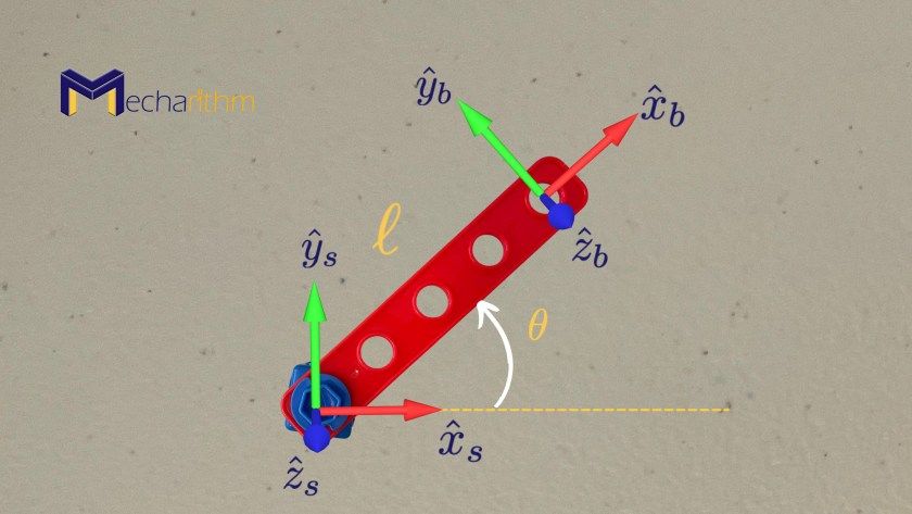
From the lesson about degrees of freedom, we learned that each rotational joint provides one rotational degree of freedom to the body that it connects. Therefore, θ is the angle of rotation about the reference configuration that is 0 at time t=0 and increases with time t. The pose of the end-effector relative to the base frame can be found using the homogenous transformation matrix T as:
The orientation of the body frame relative to the space frame can easily be expressed as the rotation matrix representing a rotation about the z-axis (please refer to the lesson about exponential coordinates of rotation and the rotation matrix lesson):
and psb(t) can be calculated from geometry as
From what we have learned so far about angular velocities and twists, we can calculate the spatial twist as:
Thus, the angular velocity expressed in the base frame can be calculated as:
And the velocity of a point currently at the origin of the {s} frame expressed in the {s} frame can be calculated as:
Therefore, the spatial twist is expressed as:
The body twist can either be calculated directly from the equations that we learned, or we can use the adjoint transformation to find the body twist as:
which can also be verified from the direct calculation. The linear part is the velocity of the origin of the body frame expressed in the body frame coordinates. θ̇ is the joint speed which shows the rate of change of the joint angle.
This can also be verified geometrically. Suppose the 1-DOF robot arm at zero configuration (note that zero configuration is shown for simplicity). The linear velocity of a point at the center of the {s} frame expressed in the {s} frame is zero since the radius of the point to the center of rotation is zero. On the other hand, the velocity of the origin of the body frame is tangent to the circular path and is at a radius of ell from the center of rotation:
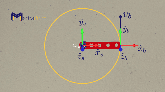
Therefore vb can be calculated as:
It was also predictable that it was in the y-direction of the {b} frame.
Example 3:
Suppose that a kid is sitting on a merry-go-round spinning counterclockwise and is at 10 cm from the center of the merry-go-round. The body frame’s x-axis is pointing outward away from the center of the table, and its y-axis is in the direction of where the kids’ eyes are looking, and the z-axis is pointing upward. The rate at which the table is rotating is 1 rad/s (θ̇ = 1). We want to find the body twist (angular velocity and linear velocity expressed in the body frame {b}). The figure below shows the sketch of the problem:
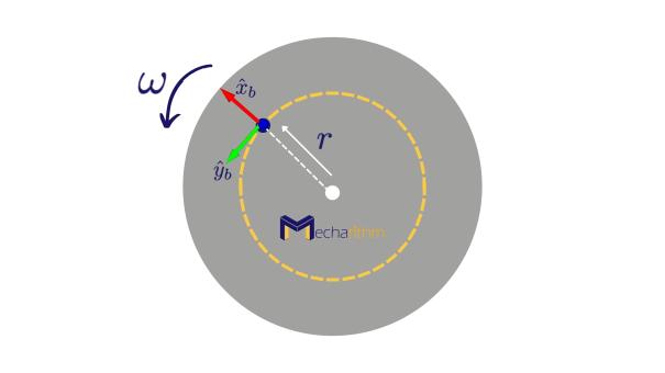
The angular velocity is in the z-direction of the body frame with the magnitude of 1 rad/s, so the body’s angular velocity is:
The linear velocity is in the direction tangent to the circular path, so we already know that it is in the body frame’s y-direction, but we can also verify that by calculation:
Imagine this linear velocity this way. During a circular motion, the centripetal force is in the direction of the center of rotation. If this force is eliminated suddenly, then the object spinning on the plate will move with that linear velocity in that direction. We already discussed this in the example of the salad spinner in the exponential coordinate of the rotation lesson.
Therefore the body twist can be expressed as:
That’s going to wrap up today’s lesson. We hope that it gave you a good understanding of velocities in robotics. In the next lesson, we will see how we can use a twist to define a screw motion. Stay Tuned! See you in the next lesson!
The video version of the current lesson can be watched at the link below:
References:
📘 Textbooks:
Modern Robotics: Mechanics, Planning, and Control by Frank Park and Kevin Lynch
A Mathematical Introduction to Robotic Manipulation by Murray, Lee, and Sastry